Introduction to the RSP Portal Aspect

Log in to the Portal Aspect by clicking on the “Portal” panel of the main landing page at data.lsst.cloud.

New for DP0.2! Image Search (ObsTAP)

The Portal’s user interface

Try it: Mouse-over text to view pop-up boxes with more detailed descriptions throughout the Portal interface. Click on any “settings” icons you see (double gears) to explore options. The Portal is a very powerful user interface with far more options than are covered in the introduction below.

“1. Select TAP Service” Leave the default (https://data.lsst.cloud/api/tap) to access DP0 data.

“2. Select Query Type” There are three types of queries: Single Table (UI assisted), Edit ADQL (advanced), and Image Search (ObsTAP). Each of these options has a different user interface, covered in the sections below.

Single Table (UI assisted)

The default query type, and default user interface, is for “Single Table (UI assisted)” queries.

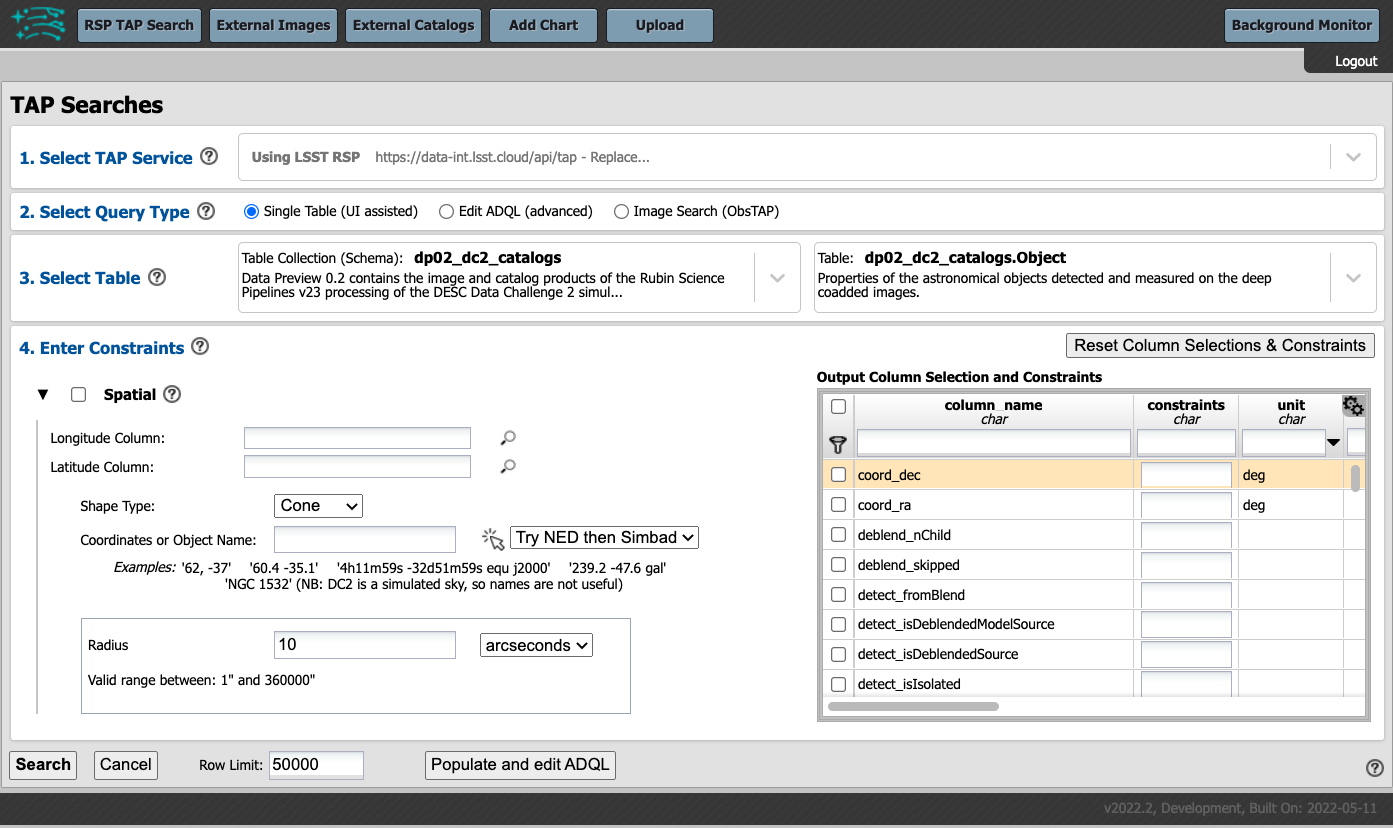
The default view of the Portal’s user interface for single table queries.

3. Select Table: Drop down menus of available tables. For DP0 data, choose the “Table Collection (Schema): dp02_dc2_catalogs” in the left drop-down menu. The default table in the right drop-down menu is the Object table. See the DP0.2 Data Products Definition Document (DPDD) for table descriptions and schema. Notice how the table view at lower-right will automatically update to match the selected table.

4. Enter Constraints: For “Spatial” constraints, the longitude and latitude columns do not yet automatically update to be the correct column names for right ascension and declination for the selected table, and need to be entered (for the Object table, they are “coord_ra” and “coord_dec”). If a non-existent column name is entered, the box will highlight red in indication of the error. Choose the desired shape type for a spatial search, such as “Cone”, and the appropriate instructions for the search terms will appear.

Keeping the search area small will keep query times short and returned manageable subsets of objects as you learn. It is recommended to start with 3 arcminutes. Note that the central coordinates for DC2, in decimal degrees, are: 61.863 -35.790.

The table view: The table to the right of “Enter Constraints” enables users to apply additional search constraints on the columns in the selected catalog table. Some tables have a lot of data columns. Search for desired data columns by entering terms (e.g., ra, Flux, or flag) in the boxes underneath “column_name” or “description” and pressing “enter” in order to view data columns of interest to you.

Use the checkboxes in the left-most column to select the data column names to be returned by the query. Use the funnel icon to filter the columns, and only view selected data column names. Use the constraints column to specify query parameters and only retrieve data which meets those constraints.

Remove filters and reset the table view at any time using the “Remove” or “Reset” buttons above the upper-right corner of the table.

ADQL conversions: If desired, convert table view queries to “ADQL Queries” using the “Populate and Edit ADQL” button at the bottom of the page. This can enable entering more complex constraints that cannot be expressed against individual columns. This will switch the user interface to the “Edit ADQL (advanced)” view.

Row limit: The “Row Limit” in the bottom bar can be changed to apply an upper bound to the number of rows returned. The Portal can work effectively with datasets with millions of rows. However, when learning or testing queries, it is advisable to limit the number of rows (e.g., 10000 rows is useful for testing).

Note: Because of the implementation of the Rubin Observatory “Qserv” database, it is not recommended to use the row limit alone in order to get a “sampling” of data. Queries with only a row limit can run for much longer than one might intuitively expect; applying a spatial constraint is likely to return a result more quickly.

Example single-table query: The image below presents and example of how to search the DP0.2 Object catalog using a 3 arcminute cone near the DC2’s central coordinates, returning only the five data columns “coord_ra”, “coord_dec”, and “g” “r” and “i_calibFlux”, and imposing the contraints that the flux must be between 20 and 1000 nanojansky (i.e., between 24th and 28th magnitude).

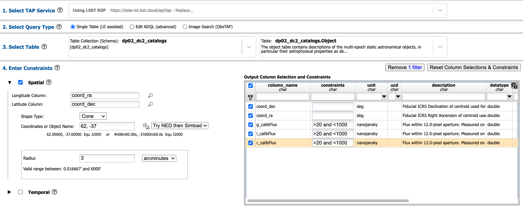
An example query of the DC2 Object catalog.

Search: Press the search button at lower left when ready to execute. The search might take a few moments.

This will show while the search is executing.

Results view: The search results will populate the results view, as shown in the figure below. There are many icons that control the display settings; hover the mouse over any of them to see a pop-up description. At upper right, notice the options “tri-view”, “img-tbl”, “img-xy”, and “xy-tbl”. The default is “tri-view”, which is shown below, with a sky image at upper left. Notice that at the time this documentation was created, the sky image was 2MASS and not a simulated DC2 image. A default “xy” plot of the sky coordinates appears at upper right, and the table of results along the bottom.

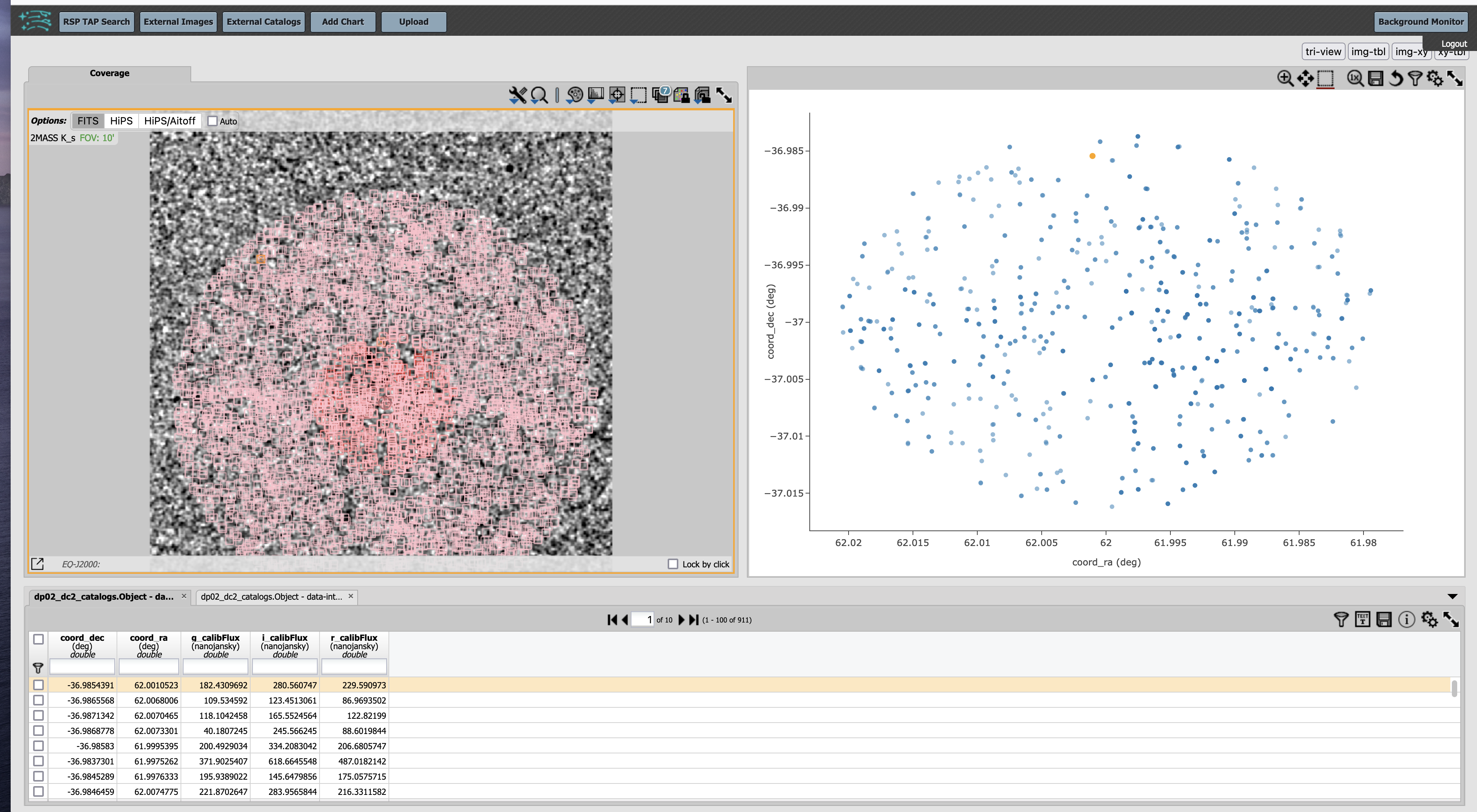
The default view of the search results.

Maniuplating the plotted data and converting fluxes to magnitudes: To manipulate the plotted data, select the double gear “settings” icon above the x-y plot and a pop-up window will open (see the next figure). To create a color-magnitude diagram from the fluxes, for DP0.2 it is necessary to apply the standard conversion from nanojansky to AB magnitude in the X and Y boxes as, e.g., “-2.5 * log10(g_calibFlux) + 31.4”. In the future, magnitudes will be available.

Add a chart title and label the axes, choose a point color, and click “Apply” and then “Close”.

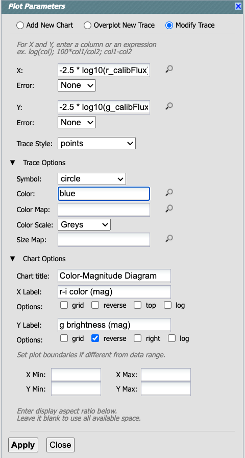
The plot settings pop-up window.

At this point, additional cuts can be applied to the table data being plotted. In the figure below, the g-band flux is limited to >100, and this imposes a sharp cutoff in the y-axis values at 26.4 mag. Select “xy-tbl” to view only the plot and the table data. Notice how the corresponding plot point for the selected row in the table is differently colored, and that hovering the mouse over the plotted data will show the x- and y-values in a pop-up window.

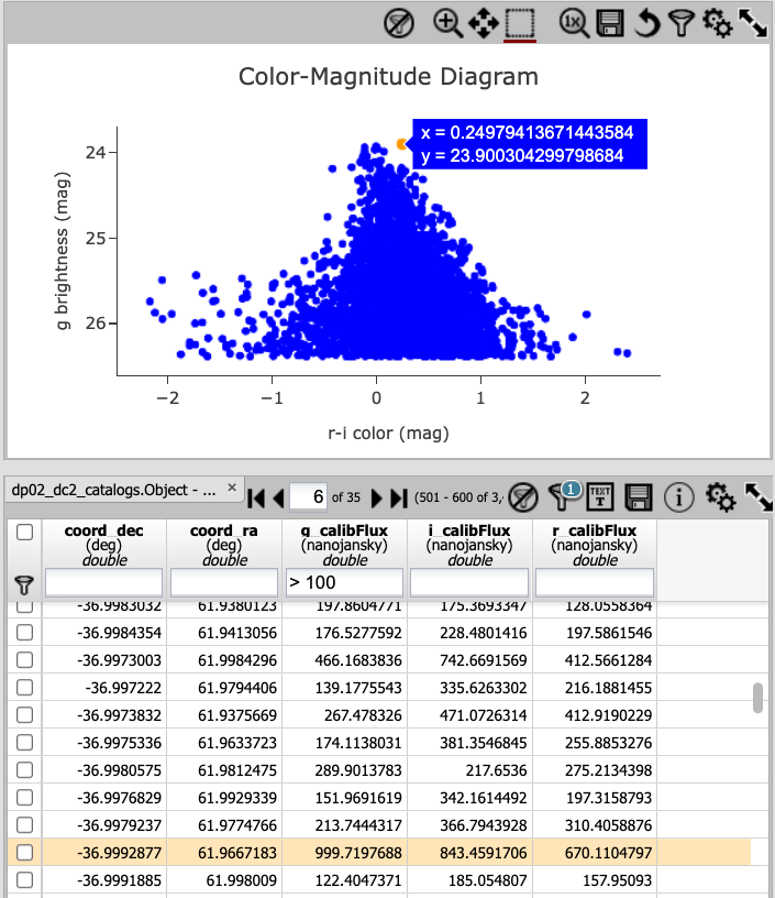
An updated results view in which the plotted data has been manipulated.

Learn more. See also Portal tutorials for additional demonstrations of how to use the Portal’s Single Table Query.

Edit ADQL (advanced)

ADQL is the Astronomical Data Query Language. The language is used by the IVOA to represent astronomy queries posted to Virtual Observatory (VO) services, such as the Rubin LSST TAP service. ADQL is based on the Structured Query Language (SQL).

Selecting “Edit ADQL (advanced)” will change the user interface to display an empty box where users can supply their query statement. Scrolling down in that interface will show several examples.

Turn a single table query into ADQL. At any point while assembling a query using the single table query interface described above, clicking on “Edit and Populate ADQL” will transform the query into ADQL. Note that any changes then made to the ADQL are not propogated back to the single table query constraints.

Converting fluxes to magnitudes is much easier with the ADQL interface by using the scisql_nanojanskyToAbMag() functionality as demonstrated below.

Query the TAP schema. Information about the LSST TAP schema can be obtained via ADQL queries. For example, to get the detailed list of columns available in the “Object” table, their associated units and descriptions:

SELECT tap_schema.columns.column_name, tap_schema.columns.unit,
tap_schema.columns.description
FROM tap_schema.columns
WHERE tap_schema.columns.table_name = 'dp02_dc2_catalogs.Object'

In the results view,

Query the Object table, as done with the single table query interface above, with the following ADQL:

SELECT coord_dec,coord_ra,g_calibFlux,i_calibFlux,r_calibFlux
FROM dp02_dc2_catalogs.Object
WHERE CONTAINS(POINT('ICRS', coord_ra, coord_dec),CIRCLE('ICRS', 62, -37, 0.05))=1
AND (g_calibFlux >20 AND g_calibFlux <1000
AND i_calibFlux >20 AND i_calibFlux <1000
AND r_calibFlux >20 AND r_calibFlux <1000)

Type the above query into the ADQL Query block and click on the “Search” button in the bottom-left corner to execute. Remember to set the “Row Limit” to be a small number, such as 10000, when testing queries. The search results will populate the same Results View, as shown above using the Single Table Query interface.

To do the same query with magnitudes:

SELECT coord_dec, coord_ra,
scisql_nanojanskyToAbMag(g_calibFlux) AS g_calibMag,
scisql_nanojanskyToAbMag(i_calibFlux) AS r_calibMag,
scisql_nanojanskyToAbMag(r_calibFlux) AS i_calibMag
FROM dp02_dc2_catalogs.Object
WHERE CONTAINS(POINT('ICRS', coord_ra, coord_dec),
CIRCLE('ICRS', 62, -37, 0.05))=1
AND scisql_nanojanskyToAbMag(g_calibFlux) < 28
AND scisql_nanojanskyToAbMag(r_calibFlux) < 28
AND scisql_nanojanskyToAbMag(i_calibFlux) < 28
AND scisql_nanojanskyToAbMag(g_calibFlux) > 24
AND scisql_nanojanskyToAbMag(r_calibFlux) > 24
AND scisql_nanojanskyToAbMag(i_calibFlux) > 24

Joining two or more tables. It is often desirable to access data stored in more than just one table. This is possible to do using a JOIN clause to combine rows from two or more tables. In the example below, the Source and CcdVisit table are joined in order to obtain the date and seeing from the CcdVisit table. Any two tables can be joined so long as they have an index in common.

SELECT src.ccdVisitId, src.extendedness, src.band,
scisql_nanojanskyToAbMag(src.psfFlux) AS psfAbMag,
cv.obsStartMJD, cv.seeing
FROM dp02_dc2_catalogs.Source AS src
JOIN dp02_dc2_catalogs.CcdVisit AS cv
ON src.ccdVisitId = cv.ccdVisitId
WHERE CONTAINS(POINT('ICRS', coord_ra, coord_dec),
CIRCLE('ICRS', 62.0, -37, 1)) = 1
AND src.band = 'i' AND src.extendedness = 0 AND src.psfFlux > 10000
AND cv.obsStartMJD > 60925 AND cv.obsStartMJD < 60955

Learn More. See also Portal tutorials for additional demonstrations of how to use the Portal’s ADQL functionality.

Image Search (ObsTAP)

The “Image Search (ObsTAP)” functionality has many new features – not just new for DP0.2, but new to the Firefly interface, and DP0 Delegates are among the first to use them.

Selecting “Image Search (ObsTAP)” will change the user interface to display query constraint options that are specific to the image data, as described below.

For more information about the image types available in the DP0.2 data set, see the DP0.2 Data Products Definition Document (DPDD).

Enter Constraints

Under “Observation Type and Source”, the IVOA standard options for “Calibration Level” (0, 1, 2, 3, or 4) are provided. For DP0.2, 1 is the raw (unprocessed) images, 2 is the processed visit images (PVIs; the calibrated single-epoch images also called calexps), and 3 are the derived image data such as difference images and deep coadds.

The “Data Product Type” should be left as “Image”, and the “Instrument Name”, “Collection”, and “Data Product Subtype” can all be left blank.

Under “Location”, only “Observation boundary contains point” was implemented at the time this documentation was written. Recall that the central coordinates for the DC2 simulated sky region is “62, -37”.

Under “Timing”, users can specify a range to apply to the image acquisition dates (this is only relvant for PVIs/calexps).

Under “Spectral”, users can provide a wavelength in, e.g., nanometers as a means of specifying the image band.

Output Column Selection and Constraints

The default is for all columns to be selected (i.e., have blue checks in the leftmost column). It is recommended to always return all metadata because the Portal requires some columns in order for the some of the Results view functionality to work.

Example (PVIs/calexps)

The image below shows an example query for all r-band PVIs (calexps) that overlap the central coordinates of DC2, which were obtained with a modified Julian date between 60000 and 60500. Note that the filter constraint is applied in the table at right, and that a subset of the most useful image metadata columns are selected.

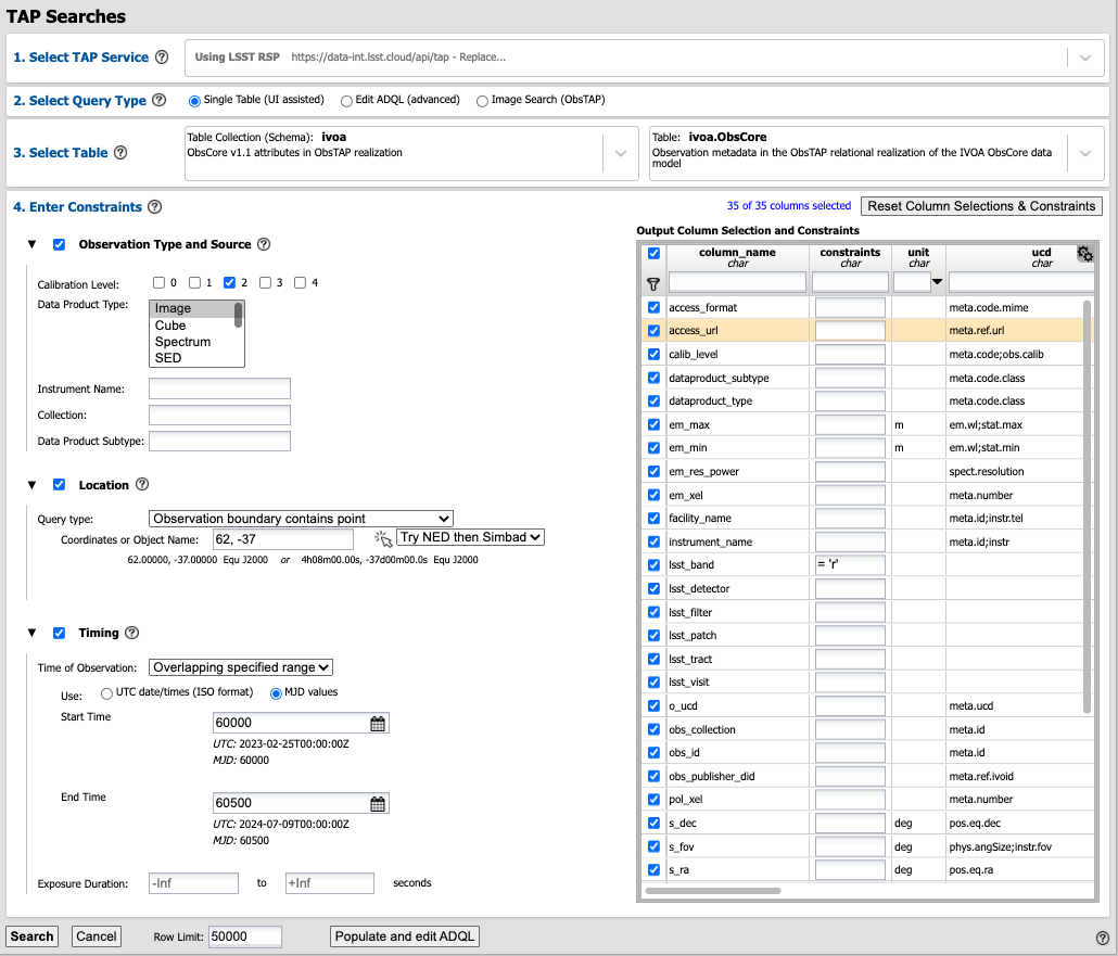
The default interface for the “Image Search (ObsTAP)” queries, with example search parameters.

Click on the “Search” button.

Results View

The default results appear in the tri-view format, with the image at upper left, an xy plot at upper right, and the table of metadata below. The first row of the table is highlighted by default, with that image showing at upper right (and the central coordinates of other images overplotted with green boxes). The xy plot default is RA versus Declination, with the location of the highlighted table row shown in orange and the rest in blue.

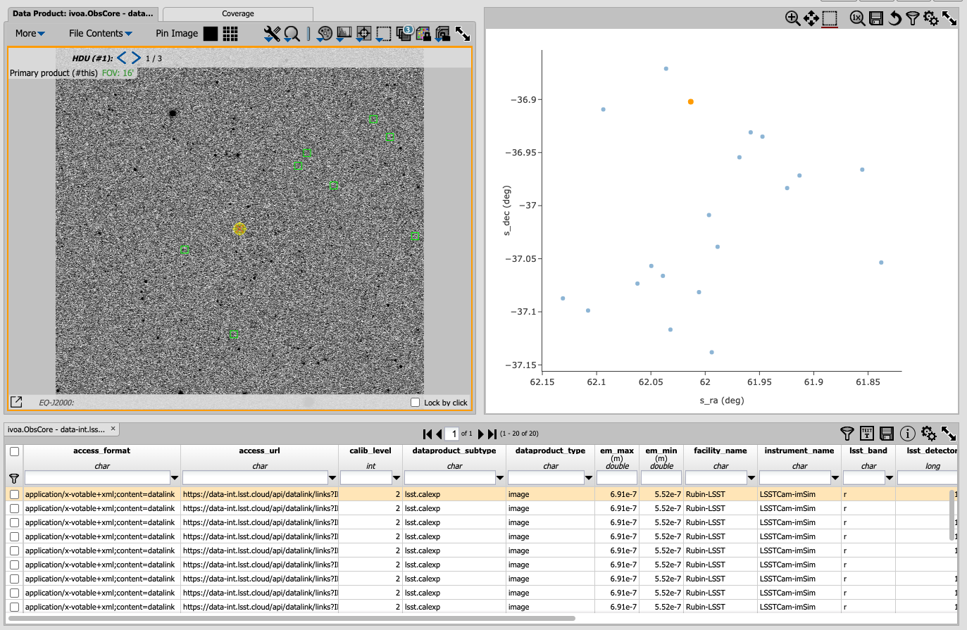
Results for the example search parameters.

Manipulating the xy plot is the same process as shown for the Single Table (UI assisted) results: click on the “settings” icon (double gears) in the upper right corner to change the column data being plotted, alter the plot style, add axes labels, etc.

Interacting with the images begins with just hovering the mouse over the image and noting the RA, Dec, and pixel value appear at the bottom. Use the magnifying glass icons in the upper left corner to zoom in and out; click and drag the image to pan. Above the magnifying glass, use the back and forth arrows to navigate between HDU (header data units) 1, 2, and 3: the image, mask, and variance data. Click either on one of the green boxes (representing the central coordinats of another image in the table), or on another row in the table, to display a different image. At upper right, click on “img-tbl” to get ride of the xy plot and show the images and the table side-by-side.

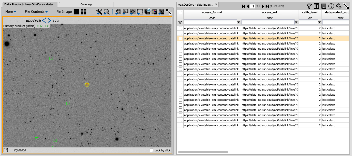
Display the image in row three of the table (with the view format set to “img-tbl”).

Image tools: There are many tools available for users, the following demonstrates use of just one. First, zoom in on a bright star in one of the images. Select the “tools” icon (wrench and ruler), and from the pop-up window choose to “Extract” using a line. Draw a line on the image across the star to extract the pixel values and show an approximate shape of the point-spread function for the star. The plot reveals that this particular star is saturated. Click on “Pin Table” to add a table of pixel data as a new tab in the right half of the view. To make the line go away, click on the “layers” icon (the one for which the hover-over text reads: “Manipulate overlay display…”) and in the pop-up window, next to “Extract Line 1 - HDU#1”, click on “Delete”.

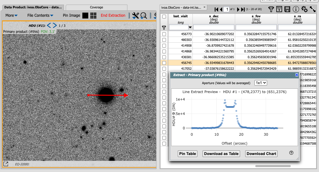
Use the image display tool to extract a line cut.

Image grid display: Above the image use the grid icon (hover-over text “Show full grid”) to show up to eight of the images side-by-side. Notice that it is possible to pan and zoom in each of these grid windows.

Coverage window: Above the image, notice that the default tab view is “Data Product…”, and instead click on “Coverage”. The bounding boxes of all images listed in the table are shown, with the image in the selected row highlighted. At the time this documentation was created, the boxes were overlayed on 2MASS images, but in the near future the background will be DC2 images.

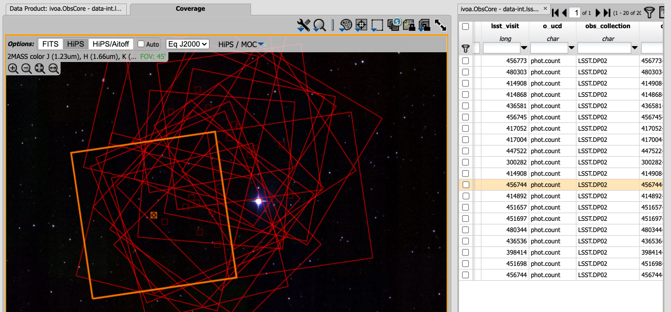
The coverage window will, in the future, be overlayed on a DC2 image and not 2MASS.

Learn More. See also Portal tutorials for a tutorial using additional image types and more of the Portal’s image-related functionality.