01. Bright Stars Color-Magnitude Diagram (beginner)
RSP Aspect: Portal
Contact authors: Melissa Graham and Greg Madejski
Last verified to run: 2024-04-30
Targeted learning level: beginner
Introduction: This tutorial uses the Single-Table Query interface to search for bright stars in a small region of sky, and then uses the Results interface to create a color-magnitude diagram. This is the same demonstration used to illustrate the Table Access Protocol (TAP) service in the first of the Notebook tutorials. Beginner-level users looking for a more general overview of the Portal Aspect should refer to this Introduction to the RSP Portal Aspect.
Step 1. Log in and set the query constraints
1.1. Log in to the Rubin Science Platform and click on Portal Aspect.
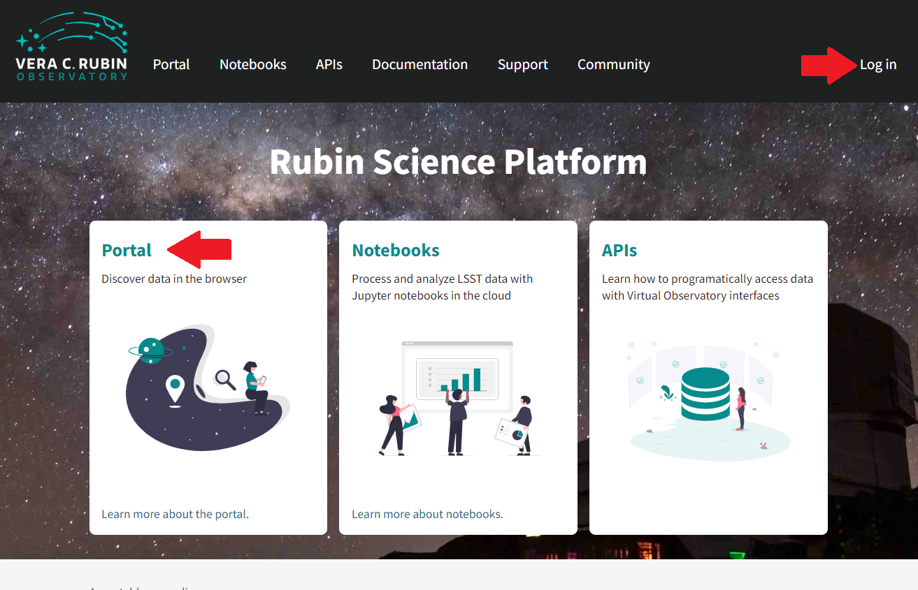
Aspect choices for the Rubin Science Platform.
1.2 On this Results tab, a temporary ‘Rubin Science Platform Portal’ graphic is shown which will later be replaced with query results, notice the tabs at the top of the screen, click on DP0.2 Catalogs to search DP02 catalogs using the Portal Aspect.
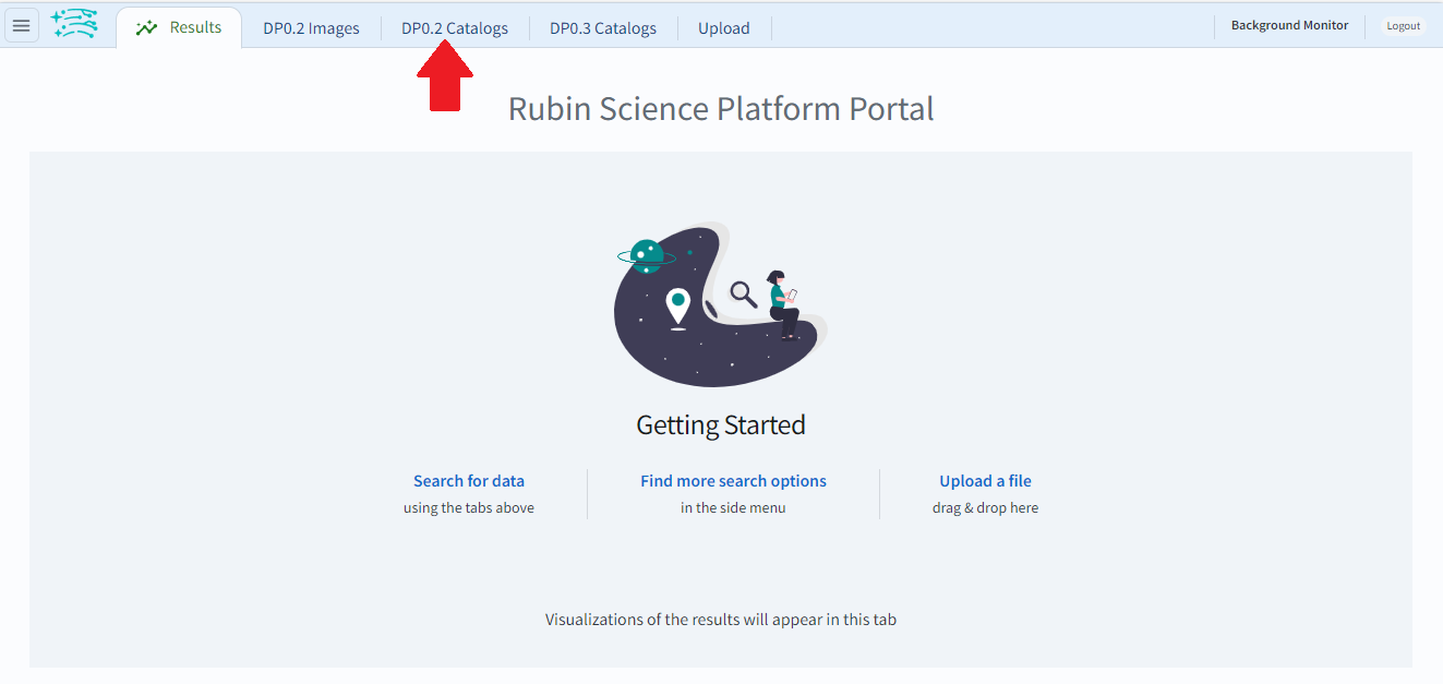
Location of tab for catalog search.
1.3. On the top left under the tab menu, under ‘LSST DP0.2 DC2 Tables’, ensure that “Use Image Search (ObsTAP)” toggle button is off (white circle to the left and grey, not white circle to the right and blue), and on the right side of the screen, leave “View” at its default “UI assisted”.
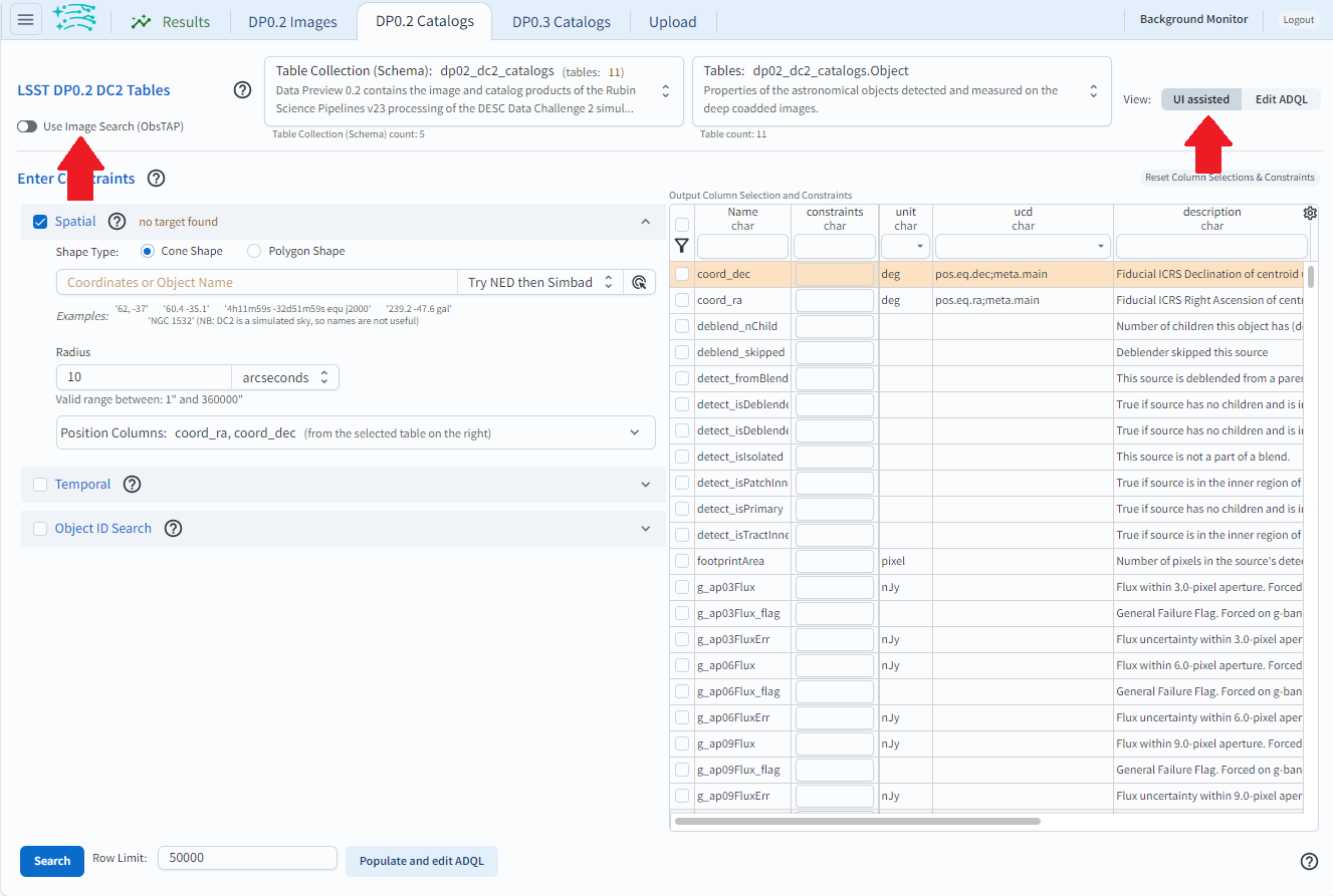
Check settings for this tutorial.
1.4. Next to “LSST DP0.2 DC2 Tables”, ensure the Table Collection says “dp02_dc2_catalogs” (left drop-down menu) and the Table is “dp02_dc2_catalogs.Object” (right drop-down menu).
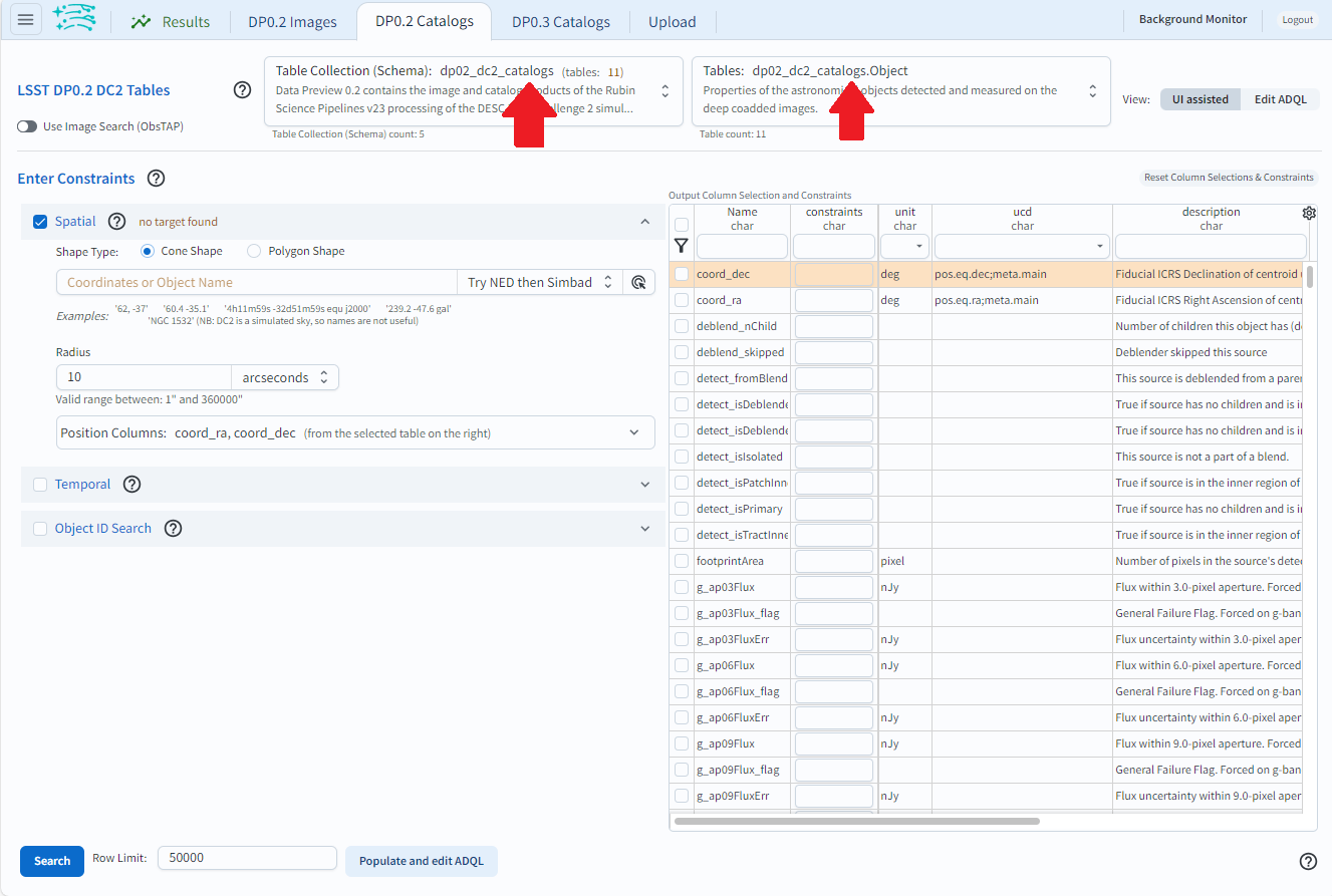
Check collection and table.
1.5. Under “Enter Constraints”, select the box to the left of “Spatial”. Leave the “Shape Type” as the default “Cone”, and for “Coordinates or Object Name” enter the central coordinates of the DC2 simulation area “62, -37”. Next to “Radius”, from the drop down menu choose “degrees” and then enter “1” in the box and press enter to set the search radius to 1 degree.
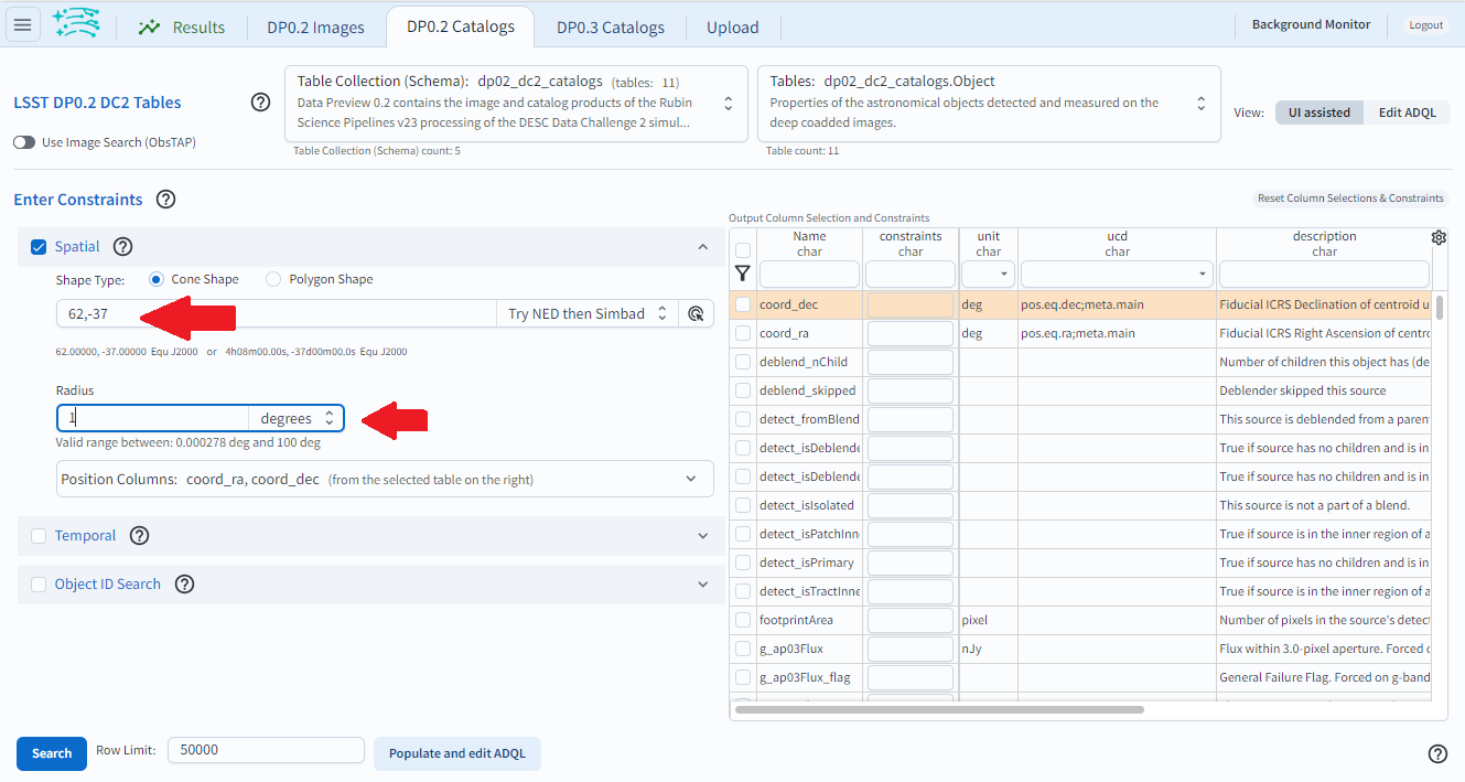
Add spatial coordinates and change the search radius.
1.6. In the table at right, under “Output Column Selection and Constraints”, click the box in the left-most column to select “coord_ra”, “coord_dec”, “detect_isPrimary”, “g” “r” and “i_calibFlux”, and “g” “r” and “i_extendedness”. Column names are searchable. To avoid scrolling a long column list, enter a keyword (e.g., “calibFlux”) in the box right below the “Name” column. It will list all the column names containing the given keyword. After selecting the needed columns (e.g., “g” “r” and “i_calibFlux”), clear the box and hit the return key to continue selecting other columns. Click on the funnel symbol at the top of the checkbox column to filter the table view to show selected columns only.
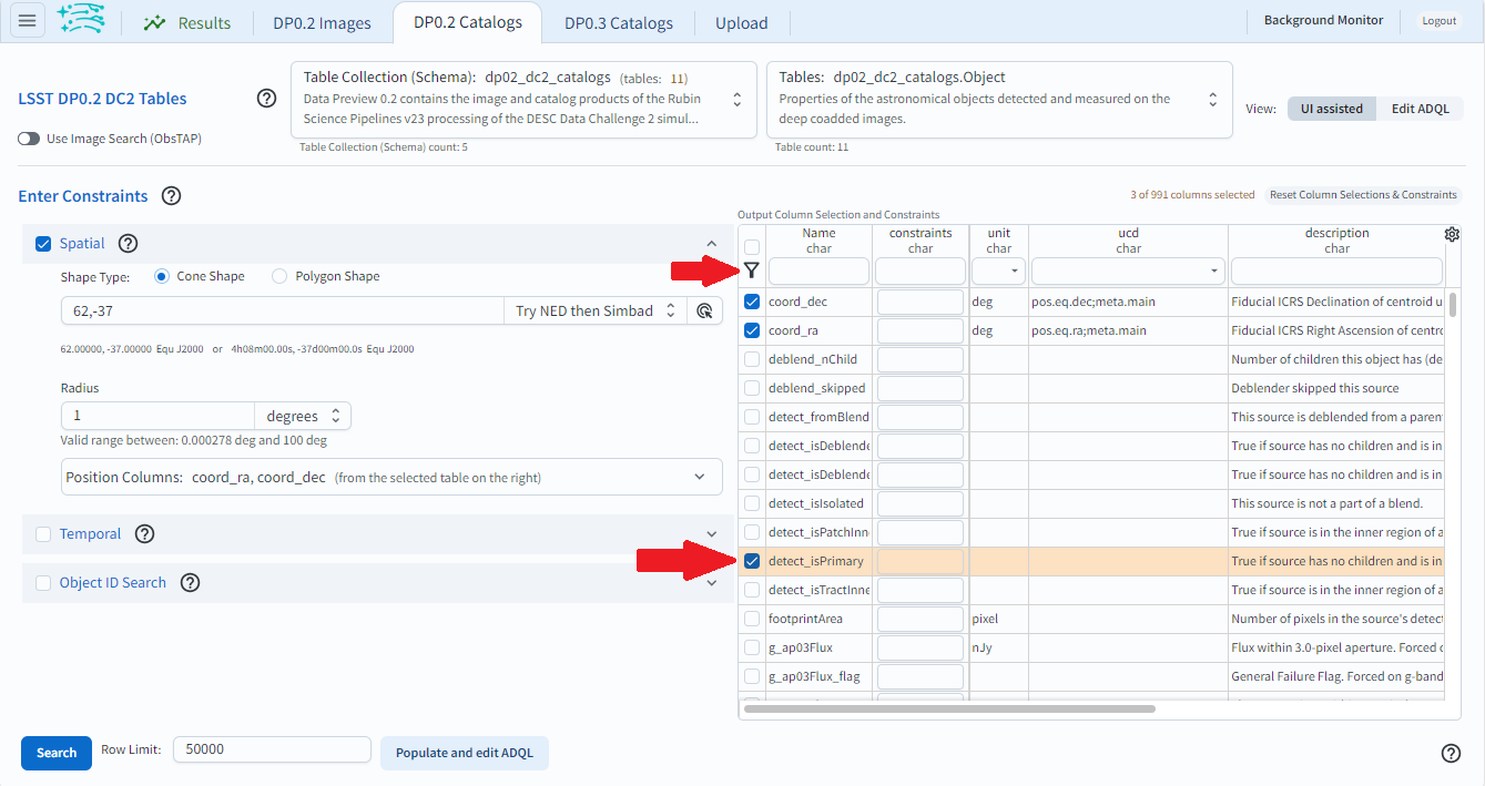
Select data to retrieve and click the filter icon.
1.7. In the “constraints” column, enter “=1” for the “detect_isPrimary”, “>360” for the fluxes, and “=0” for the extendedness parameters. (See image in step 1.8). This will limit the objects returned to those with no children (i.e., the products of deblending), which are brighter than about 25th magnitude in the g, r, and i filters, and which appear to be point-like (not extended, but not necessarily stellar) in those three filters as well.
At this point the boxes selecting the “extendedness” and “detect_isPrimary” parameters can be unchecked, because it is not necessary for this tutorial to actually retrieve the data in those columns, only to constrain the query based on their values.
Notice: At this point, with the query all set up, clicking “Populate and Edit ADQL” will switch the Query Type to “Edit ADQL” and populate the ADQL query box, as shown in Step 3 below.
1.8. Set the “Row Limit” to 10000, to only retrieve 10,000 objects for this demonstration.
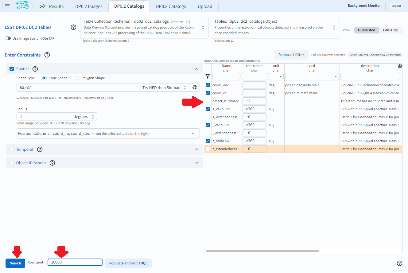
The above screenshot shows the constraints before clicking “Search”.
1.9. Click “Search” at lower left.
Step 2. Create the color-magnitude diagram
The default layout shows a sky coverage map from DESC DC2 simulation at upper left, an active chart showing the spatial distribution of returned objects at upper right, and a table of the search results along the bottom. To change the layout displayed on the screen, click the hamburger icon at the top left.
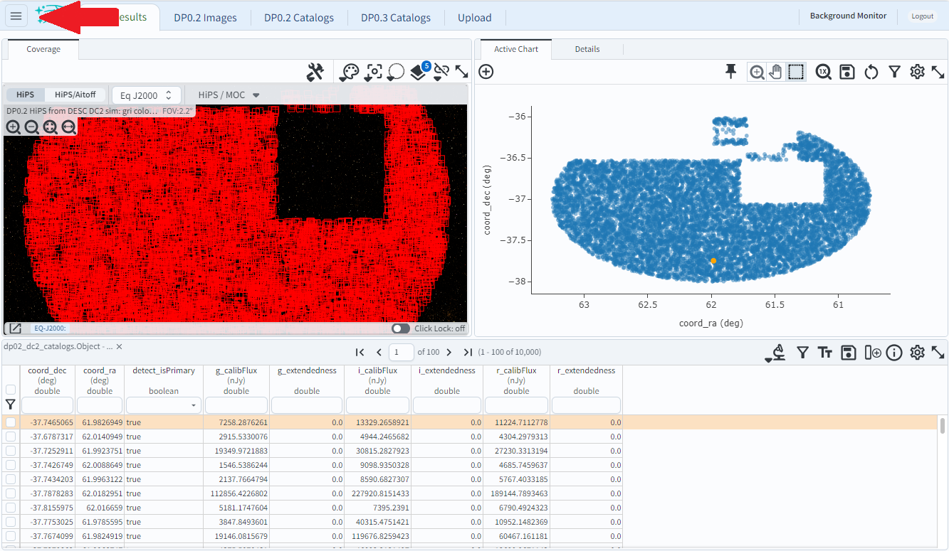
The default Results view with initial view.
2.1. Scroll down to ‘Results Layout’, and click the double arrow to get a selection of layouts for the result. For this step in this tutorial, select ‘Tables/Coverage Charts” option. Toggle between “Active Chart” and “Coverage” on the tab in the right side image box.
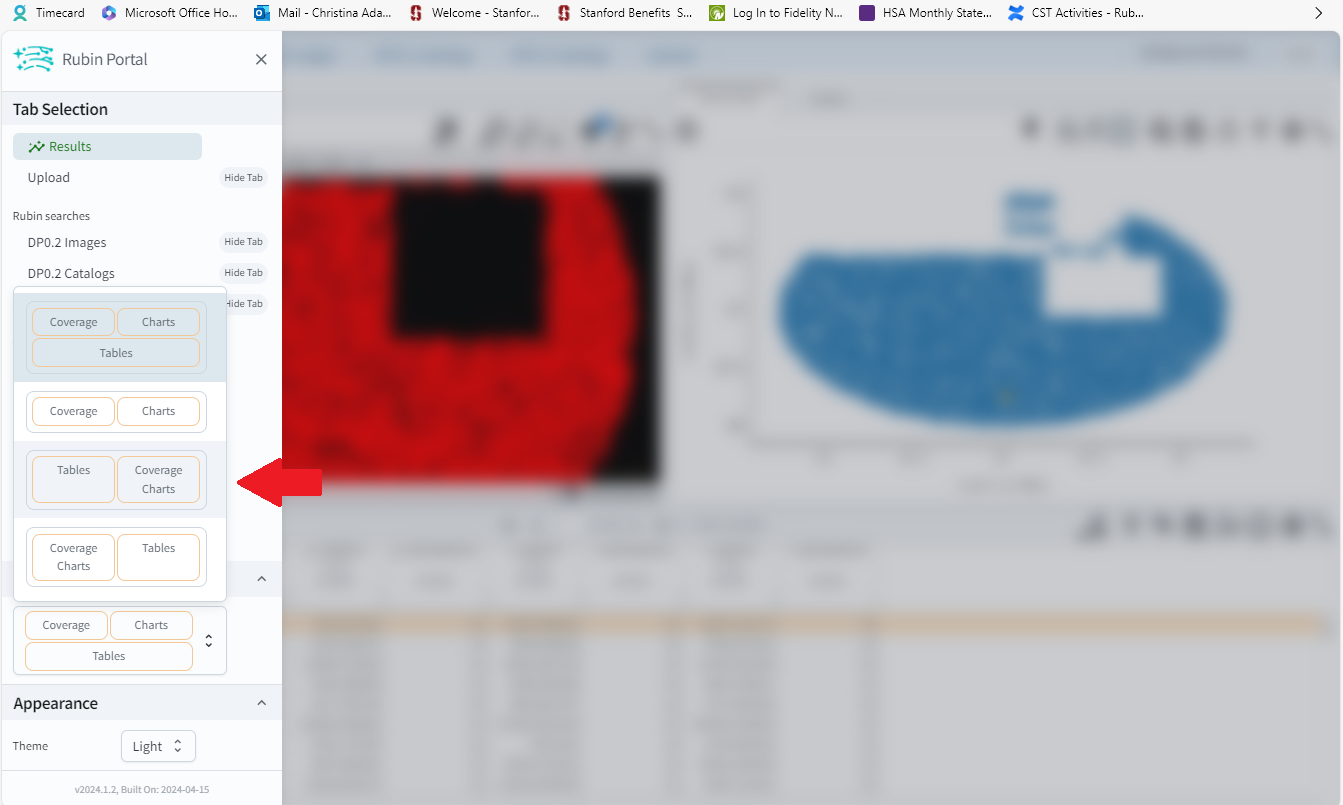
Change the layout of the query results.
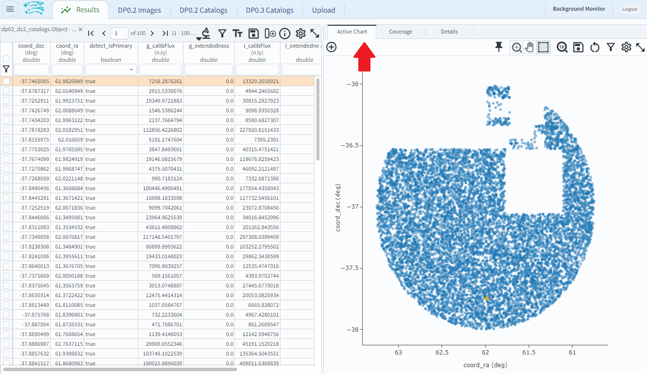
Switch between coverage and active chart.
Notice: The objects retrieved do not fill in the search area (a 1 degree radius) in the default active chart of “coord_ra” versus “coord_dec”. This is because a row limit of 10,000 objects was applied, and the data is partitioned into files by sky coordinate. The query accessed these files until 10,000 objects were found (i.e., the query does not find all objects that satisfy the query parameters and then choose 10,000 random objects to return).
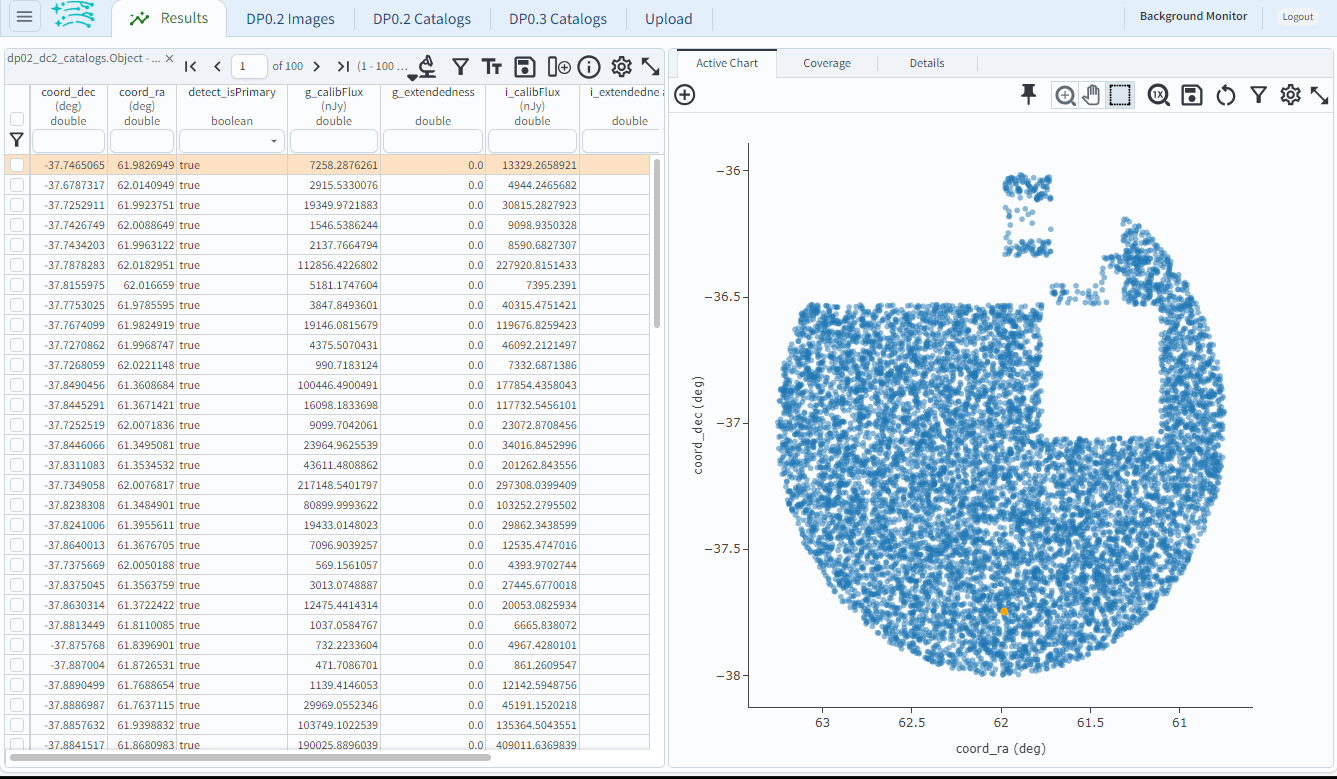
The Results view with table and coverage charts selected.
Notice: In order to plot color (r-i magnitude) versus magnitude (g), the fluxes (which are in units of nanojansky) are being converted to AB magnitudes in the next step. The AB Magnitudes Wikipedia page provides a concise resource for users who are unfamiliar with AB magnitudes and fluxes in units of janskys.
2.2. Click on the Active Chart settings icon (one gear, upper right corner of the right hand image) in order to “modify trace”, which means to change the plot parameters. Set “X” to be “(-2.5 * log10(r_calibFlux)) - (-2.5 * log10(i_calibFlux))”, and “Y” to be “-2.5 * log10(g_calibFlux) + 31.4”. Leave the options on “Trace Options” as they are, and click on “Chart Options” to show the options. For “Chart title” enter “Color-Magnitude Diagram”; set “X Label” to “color (r-i)”; set “Y Label” to “magnitude (g)”, and underneath check the “Options” box for “reverse”. Input the “X Min/Max” values “-0.5” and “2.0”, and the “Y Min/Max” values to “16.5” and “25.5” in the respective boxes.
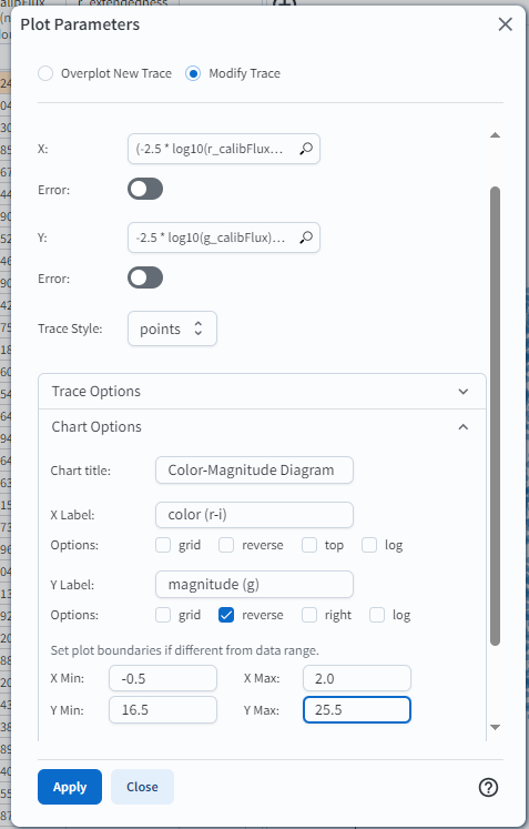
Set the plot parameters.
2.3. Click “Apply” and look at the color-magnitude plot.
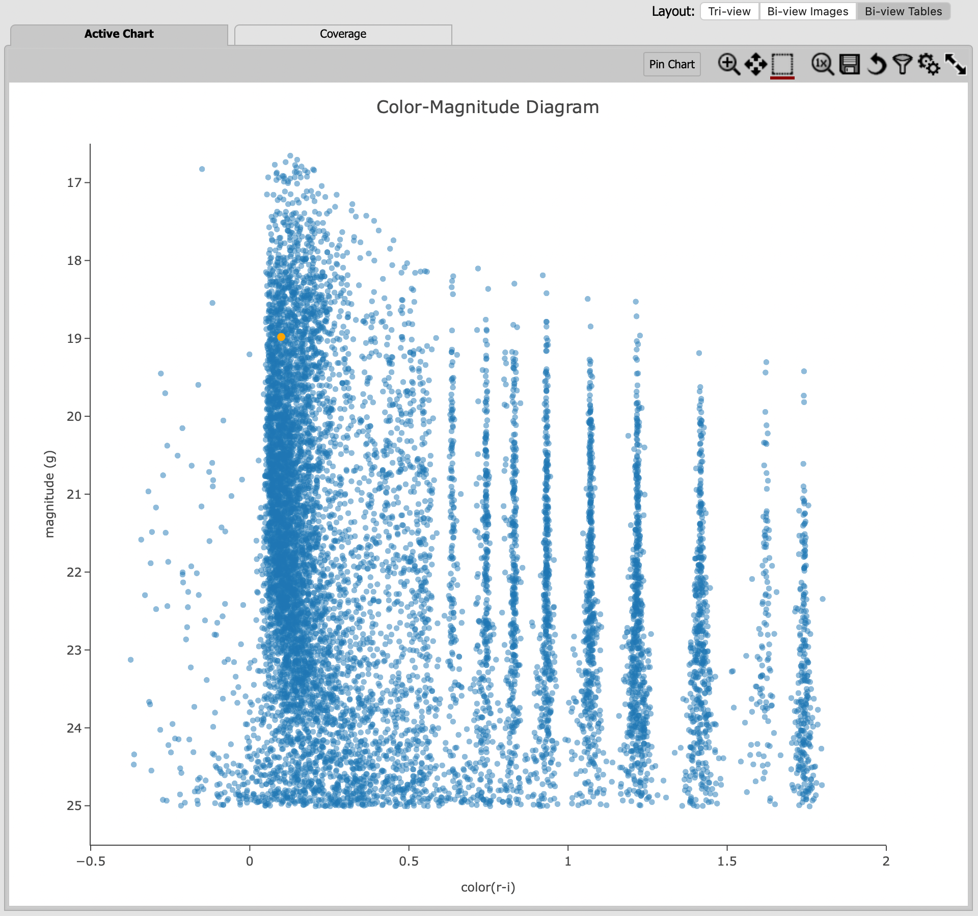
The color-magnitude diagram.
Notice: The default plot style is a scatter plot, which is appropriate for our data set of a modest size (such as 10,000 objects retrieved here). It is also possible to create a two-dimensional histogram, appropriate for large data sets (a “heat map”) which we will make in Step 2.4.
Notice: The simulated data is visibly quantized in the above plot, and this will not be the case with real data. The discrete sequences at red colors, (g-i) > 0.5, come from the discretized procedure used to simulate low-mass stars in the DP0.2 data set.
2.4. Click on the plus symbol in the upper left corner of the Color-Magnitude Diagram to “Add New Chart.” Change the “Plot Type” from “Scatter” to “Heatmap”, and then set the “X” and “Y” to the same equation as in Step 2.2. Use the same “Chart Options” except give it a different “Chart title”, such as “Heatmap Color-Magnitude Diagram.”
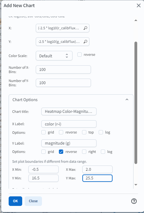
Above, we set the new chart parameters for a heatmap plot.
2.5. Click “Okay” and look at the new color-magnitude plot. Resize the “Active Charts” area to expand the plots and minimize the “Coverage” window. For completeness, you might wish to update the title of the plot you generated previously to “Scatter Color-Magnitude Diagram.”
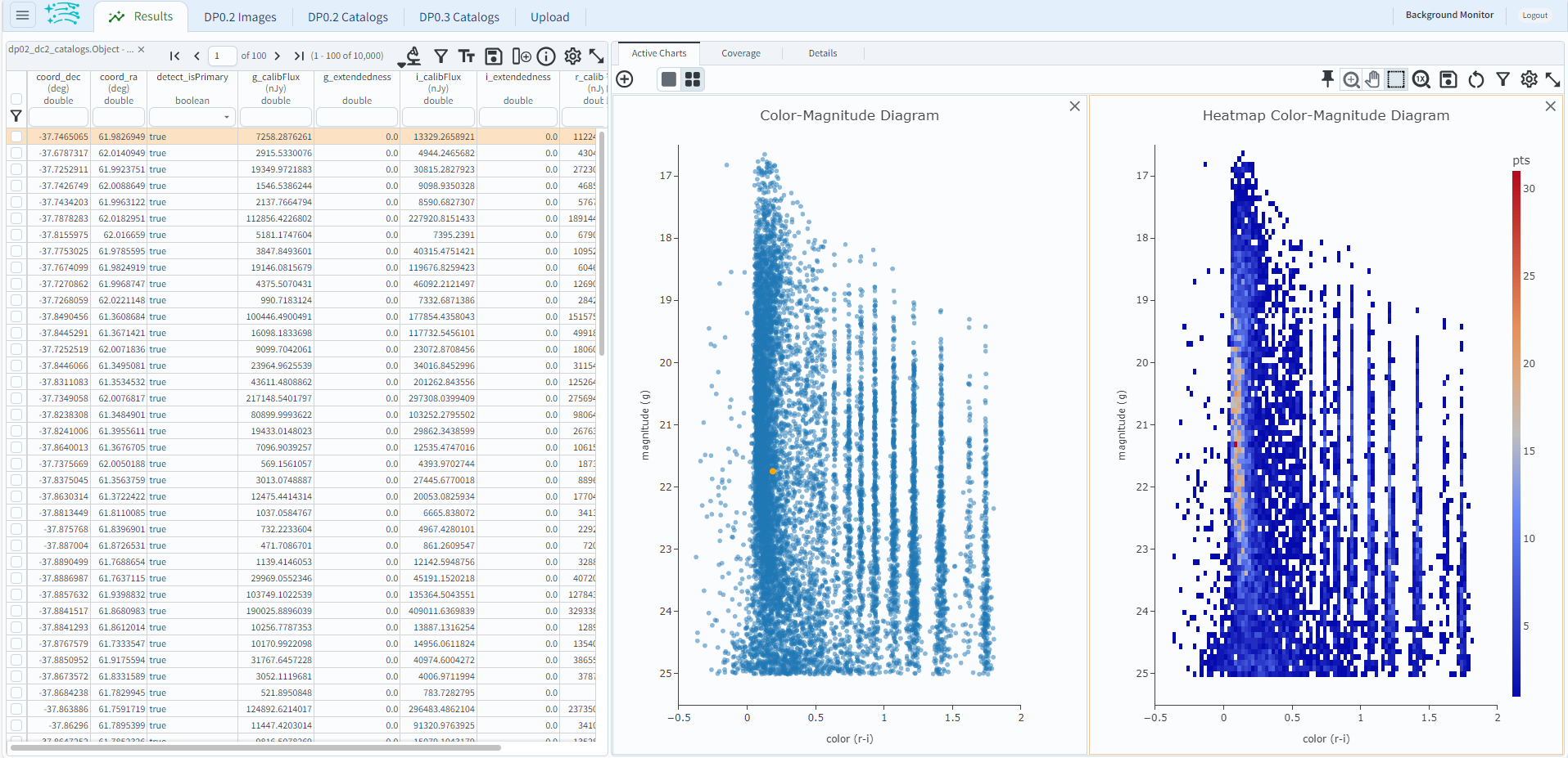
The color-magnitude diagrams, including the previously made scatter plot (left) and the heatmap (right).
2.6. Interact with the plot. Hover over the data points with a mouse either on the Coverage map (see the coordinates change in the bottom of the map) or the Active Chart (see the x and y values appear in a pop-up window). Select a row in the table and it appears as a different color in the plot(s), and vice-versa: select a point in a plot and it is highlighted in the table below.
Step 3. Do the same query with ADQL
3.1. Click on the DP0.2 Catalogs tab to return to the Portal screen. In the upper right, select “Edit ADQL” for “View”, and enter the following in the box under “ADQL Query”.
SELECT coord_dec,coord_ra,g_calibFlux,i_calibFlux,r_calibFlux
FROM dp02_dc2_catalogs.Object
WHERE CONTAINS (POINT('ICRS', coord_ra, coord_dec), CIRCLE('ICRS', 62.0, -37.0, 1)) = 1
AND detect_isPrimary =1
AND g_calibFlux >360 AND g_extendedness =0
AND i_calibFlux >360 AND i_extendedness =0
AND r_calibFlux >360 AND r_extendedness =0
3.2. At the bottom of that page, set the “Row Limit” to 10000 and then click “Search” at lower left. The Portal will transition to the “Results Tab” as in Step 2, above.
Notice: Although the same “Row Limit” of 10,000 was applied both in Step 1.7 and Step 3.2, the two searches will not return the exact same rows. Queries which return only a subset of all possible results, in this case 10,000 out of all possible rows, will return random subsets.
Step 4. Transfer ADQL queries or results from the Portal to the Notebook Aspect
4.1. As described under Step 1.6, once a query is all set up in the Portal using the “UI assisted”, click “Populate and Edit ADQL” to switch the Query Type to “Edit ADQL” and populate the ADQL query box. Shown below is the same query as in Step 3.1 above:

To execute the query in the Portal, click the “Search” button.
To execute the query in the Notebook Aspect, copy-paste the ADQL statement into the code cell of any notebook that which uses the TAP service, as demonstrated in Section 2.3 of the first tutorial notebook, 01 Introduction to DP0.2.
4.2. It is also possible to obtain a URL for direct access to the query results. This URL can be used from the Notebook Aspect; this is an especially useful feature for queries that are large, complex, or time-consuming to execute (for instance, multiple table joins), or for sharing query results with colleagues. (Note - the screenshot is an older version of the RSP, but the functionality remains the same.)
As an example, the image below displays the Results View for a small query using just a 0.05 degree radius.
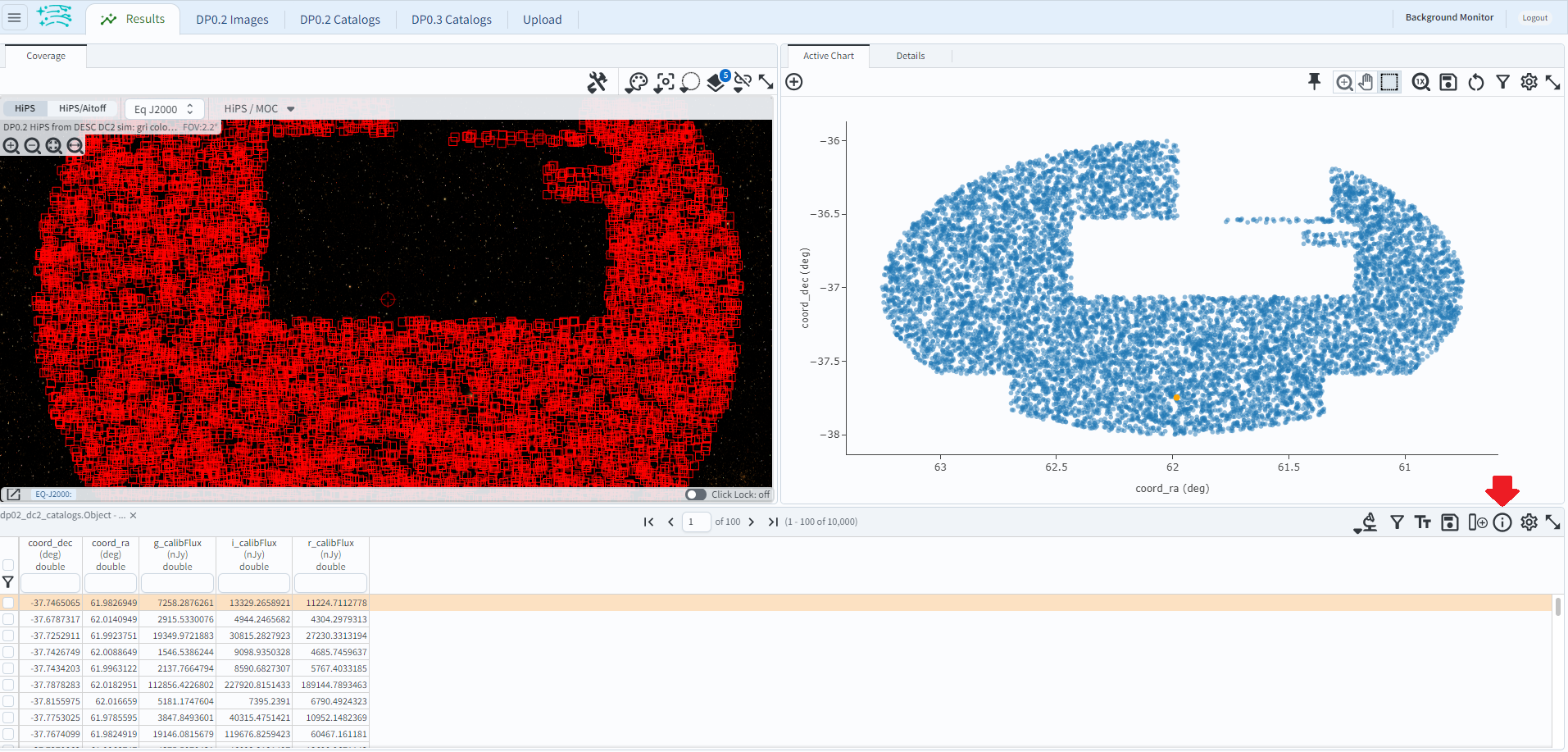
Click on the “info” button (letter “i” in a circle), and a pop-up window will appear:
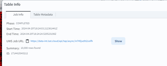
The “UWS JOB URL” in the pop-up is the URL to the query results. Click on the clipboard icon to copy the URL to your clipboard.
As demonstrated in Section 5.4 of the second tutorial notebook, 02 Catalog Queries with TAP, the URL can be pasted into a code cell and the query results retrieved using the following commands:
retrieved_job = retrieve_query('my_portal_url')
retrieved_results = retrieved_job.fetch_result().to_table().to_pandas()
This results in having the same data in your notebook which you first obtained via the Portal Aspect.
We note that URLs will not be accessible indefinitely, but rather are intended to serve the use case of immediate access and analysis. To preserve and recreate queries at a later date, it is recommended to save the ADQL-formatted query as described in step 1.6.