Contact author: Melissa Graham, Aaron Meisner
Last verified to run: 2024-10-21
LSST Science Pipelines version: Weekly 2022_40
Container Size: large
Targeted learning level: advanced
WARNING: This notebook will only run with LSST Science Pipelines version Weekly 2022_40.
To find out which version of the LSST Science Pipelines is being used, look in the footer bar or execute the cell below.
! echo $IMAGE_DESCRIPTION
Weekly 2022_40
If Weekly 2022_40 is being used, then proceed with executing the tutorial.
If Weekly 2022_40 is not being used, log out and start a new server:
Weekly 2022_40.NOTICE:
This notebook will only run with the butler repo alias dp02-direct.
All other tutorial notebooks in this repository use the dp02 alias, which was updated in Oct 2024 to provide
read-only access to butler data repos.
As this tutorial writes processed images back to the butler, "direct access" is needed and dp02-direct must be used.
Note that this is a temporary work around for Data Preview 0.
Butler functionality for Data Preview 1 will be different, as the butler service continues to evolve.
Description: Detect and measure sources in a custom "deepCoadd" image.
Skills: Use the butler and LSST pipeline tasks on user-generated collections. Run source detection, deblending, and measurement.
LSST Data Products: user-generated deepCoadd; DP0.2 deepCoadd image and Object table
Packages: lsst.afw, lsst.pipe, lsst.ctrl
Credit: Originally developed by Melissa Graham and Clare Saunders, this tutorial draws on the contents of the "Introduction to Source Detection" DP0.2 tutorial notebook by Douglas Tucker and Alex Drlica-Wagner.
Get Support: Find DP0-related documentation and resources at dp0-2.lsst.io. Questions are welcome as new topics in the Support - Data Preview 0 Category of the Rubin Community Forum. Rubin staff will respond to all questions posted there.
WARNING: This tutorial uses the output of notebook DP02_09a_Custom_Coadd.ipynb. Users must run that notebook first, or have already generated the relevant custom coadd from the command line as in DP0.2 command line tutorial 02.
This tutorial notebook is a follow-up to DP02_09a_Custom_Coadd.ipynb, and demonstrates how to run source detection and measurement on a user-generated custom deepCoadd image.
Recall that although that new custom deepCoadd is not actually deep, but a rather shallower custom coadd, it will still be called deepCoadd in the butler because that is the default name of results from the assembleCoadd task.
import getpass
import numpy as np
import matplotlib.pyplot as plt
from astropy.wcs import WCS
from astropy.coordinates import SkyCoord
import astropy.units as u

import lsst.geom
from lsst.daf.butler import Butler
from lsst.rsp import get_tap_service
import lsst.afw.display as afwDisplay

from lsst.ctrl.mpexec import SimplePipelineExecutor
from lsst.pipe.base import Pipeline
Set afwDisplay to use a matplotlib backend.
afwDisplay.setDefaultBackend('matplotlib')
Instantiate the TAP service, which is used in Section 3.3.
tap_service = get_tap_service()
Create a temporary butler in order to identify the collection and run containing the custom deepCoadd.
my_username = getpass.getuser()
butler_repo = 'dp02-direct'
tempButler = Butler(butler_repo)
Print all collections and runs associated with the current user's username.
for c in sorted(tempButler.registry.queryCollections('*'+my_username+'*')):
    print(c)
u/melissagraham/custom_coadd_window1_cl00
u/melissagraham/custom_coadd_window1_cl00/20230522T024824Z
u/melissagraham/custom_coadd_window1_cl00/20231107T001052Z
u/melissagraham/custom_coadd_window1_cl00_det
u/melissagraham/custom_coadd_window1_cl00_det/20231107T051840Z
u/melissagraham/custom_coadd_window1_test1
u/melissagraham/custom_coadd_window1_test1/20230413T030012Z
u/melissagraham/custom_coadd_window1_test1/20240418T162549Z
u/melissagraham/custom_coadd_window1_test1_nbdet/20231127T182303Z
u/melissagraham/custom_coadd_window1_test1_nbdet/20240422T020724Z
u/melissagraham/custom_coadd_window1_test2
u/melissagraham/custom_coadd_window1_test2/20241021T182310Z
u/melissagraham/custom_coadd_window1_test3
u/melissagraham/custom_coadd_window1_test3/20241018T231407Z
u/melissagraham/injection_inputs21_contrib
u/melissagraham/test0_injection_inputs
u/melissagraham/test2_injection_inputs
u/melissagraham/test_injection_inputs
u/melissagraham/test_injection_inputs_240426_1
u/melissagraham/test_injection_inputs_240426_2
u/melissagraham/test_injection_inputs_V2
u/melissagraham/test_injection_inputs_v2
Delete this temporary butler.
del tempButler
Create a new butler with the collection containing the custom deepCoadd.
Stop! Make sure the name of the collection below matches the name of the collection created when running tutorial notebook DP02_09a_Custom_Coadd.ipynb, or when executing DP0.2 command line tutorial 02.
inputCollection = "u/"+my_username+"/custom_coadd_window1_test2"
print(inputCollection)
u/melissagraham/custom_coadd_window1_test2
butler = Butler(butler_repo, collections=[inputCollection])
Use the dataId from tutorial notebook DP02_09a_Custom_Coadd.ipynb and retrieve the custom deepCoadd.
my_dataId = {'band': 'i', 'tract': 4431, 'patch': 17}
my_deepCoadd = butler.get('deepCoadd', my_dataId)
Confirm that the retrieved deepCoadd is the custom user-generated 6-input visits version.
my_deepCoadd_inputs = my_deepCoadd.getInfo().getCoaddInputs()
my_deepCoadd_inputs.visits.asAstropy()
| id | bbox_min_x | bbox_min_y | bbox_max_x | bbox_max_y | goodpix | weight | filter |
|---|---|---|---|---|---|---|---|
| pix | pix | pix | pix | ||||
| int64 | int32 | int32 | int32 | int32 | int32 | float64 | str32 |
| 919515 | 11900 | 7900 | 16099 | 12099 | 8982709 | 3.4656688819793495 | i_sim_1.4 |
| 924057 | 11900 | 7900 | 16099 | 12099 | 16098179 | 4.384267091685517 | i_sim_1.4 |
| 924085 | 11900 | 7900 | 16099 | 12099 | 831332 | 4.446833161599578 | i_sim_1.4 |
| 924086 | 11900 | 7900 | 16099 | 12099 | 16136708 | 4.550420295334223 | i_sim_1.4 |
| 929477 | 11900 | 7900 | 16099 | 12099 | 16280498 | 4.051326013718346 | i_sim_1.4 |
| 930353 | 11900 | 7900 | 16099 | 12099 | 16076133 | 3.7685753871220466 | i_sim_1.4 |
This tutorial uses an approach to running source detection that is meant to parallel the approach adopted in tutorial notebook 09a for coaddition: use the Simple Pipeline Executor to run a subset of Tasks from the DP0.2 Data Release Production (DRP) pipeline. The usage of SimplePiplineExecutor here also closely parallels the command line version of source detection demonstrated in DP0.2 command line tutorial 02.
For technical reasons, it's necessary to use a collection other than the input collection for the source detection outputs. Define an output collection name into which the custom coadd source detection results will be persisted:
my_outputCollection_identifier = 'custom_coadd_window1_test2_nbdet'
my_outputCollection = 'u/' + my_username + '/'+ my_outputCollection_identifier
print(my_outputCollection)
u/melissagraham/custom_coadd_window1_test2_nbdet
As in the DP0.2 custom coaddition tutorial, the next step is to define a "simple butler" object that will be needed for running the SimplePipelineExecutor:
simpleButler = SimplePipelineExecutor.prep_butler(butler_repo,
                                                  inputs=[inputCollection],
                                                  output=my_outputCollection)
Below, check that the newly created output collection is first in the list.
Notice: A run timestamp has been added to
my_outputCollectionas additional information for users.
Warning: To run custom coadd source detection multiple times, identify each source detection deployment with a new output collection name, such as
custom_coadd_window1_test1_nbdet2orcustom_coadd_window1_test1_nbdet3, and so on.
Note that re-executing Section 2.4 with the same output collection name will produce results with a new run timestamp, but the butler always retrieves data from the most recent timestamp for a given collection. Not setting a new output collection name for a new deployment of source detection is essentially like "overwriting" results in the butler. It is not recommended to work that way, but to bookkeep using output collection names.
simpleButler.registry.getCollectionChain(my_outputCollection)
CollectionSearch(('u/melissagraham/custom_coadd_window1_test2_nbdet/20241021T190312Z', 'u/melissagraham/custom_coadd_window1_test2'))
Now for the pipeline definition. Use a subset of the pipeline Tasks from the DP0.2 DRP pipline, which is defined by the $DRP_PIPE_DIR/pipelines/LSSTCam-imSim/DRP-test-med-1.yaml YAML file. Specifically, four "steps" from within the DP0.2 DRP pipeline will be run: (1) detection, the initial detection of sources within the custom coadd (2) mergeDetection, which is needed to make possible downstream processing steps (3) deblend, deblending based on further analysis of the initial detection list (4) measure, which computes useful quantities, such as the photometric fluxes, given the deblended list of sources.
As in DP0.2 notebook tutorial 09a, it's necessary to combine this information about the pipeline definition YAML file name and the desired subset of pipeline steps. This is done by creating a Uniform Resource Identifier (URI) containing all of this relevant information as follows:
yaml_file = '$DRP_PIPE_DIR/pipelines/LSSTCam-imSim/DRP-test-med-1.yaml'
steps = 'detection,mergeDetections,deblend,measure'
my_uri = yaml_file + '#' + steps
print(my_uri)
$DRP_PIPE_DIR/pipelines/LSSTCam-imSim/DRP-test-med-1.yaml#detection,mergeDetections,deblend,measure
Note how the URI begins with the full DP0.2 DRP YAML pipeline definition file name, then, after a # character, continues with a comma-separated list of the desired pipeline steps. The order in which these steps are listed after the # character does not matter, though here they are listed in the order they run during processing for the sake of understandability.
Now create a source detection pipeline object based on the URI just constructed:
sourceDetectionPipeline = Pipeline.from_uri(my_uri)
As in DP0.2 tutorial notebook 09a, it's necessary to apply a small number of configuration overrides to customize the pipeline's operation. The first two configuration overrides below set the detection threshold applied to the custom i-band coadd to be 10 sigma. The 10 sigma detection threshold employed here is used only for the sake of an additional configuration override example, but should not be interpreted as a general-purpose recommendation. The multibandDeblend.maxIter configuration override sets the maximum deblending iterations to a lower value than its default, which is a recommended mechanism for speeding up the processing. The doPropagateFlags configuration override is set because this processing does not need to propagate flag information about which sources were used for PSF construction.
sourceDetectionPipeline.addConfigOverride('detection', 'detection.thresholdValue', 10.0)
sourceDetectionPipeline.addConfigOverride('detection', 'detection.thresholdType', "stdev")
sourceDetectionPipeline.addConfigOverride('deblend', 'multibandDeblend.maxIter', 20)
sourceDetectionPipeline.addConfigOverride('measure', 'doPropagateFlags', False)
QuantumGraph¶Recall that the QuantumGraph is a tool used by the LSST Science Pipelines to break a large processing into relatively “bite-sized” quanta and arrange these quanta into a sequence such that all inputs needed by a given quantum are available for the execution of that quantum. In the present case, the processing is not especially large, but for production deployments it makes sense to inspect and validate the QuantumGraph before proceeding straight to full-scale processing launch. The image below provides a visualization of the custom coadd processing's QuantumGraph.
Here's what the QuantumGraph for the pipeline to perform source detection, debleding, and measurement looks like:
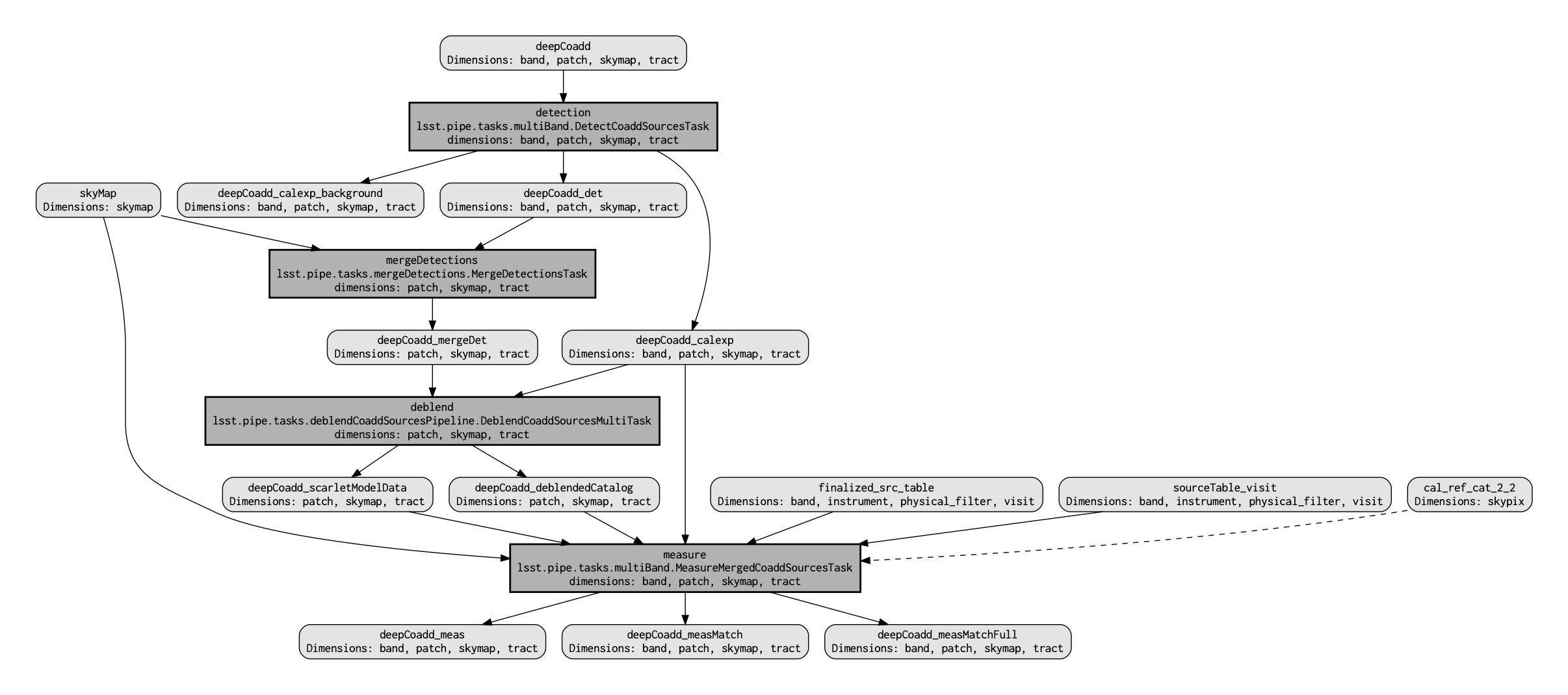
The pipeline workflow starts from the top of the QuantumGraph, the custom deepCoadd, and works its way down to the bottom, where one can see that the final output data products (light gray rectangles with rounded corners) arise from the measure Task
Option: to recreate the above QuantumGraph visualization, uncomment the following cell and run it. Note that running the following optional commands will create two files, source_detection_qgraph.dot and source_detection_qgraph.png, in the current user's RSP home directory. Note also that running this optional QuantumGraph recreation will yield a warning message which can be ignored.
#from lsst.ctrl.mpexec import pipeline2dot
#pipeline2dot(sourceDetectionPipeline, '/home/' + my_username + '/source_detection_qgraph.dot')

#! dot -Tpng /home/$USER/source_detection_qgraph.dot > /home/$USER/source_detection_qgraph.png
Important: The goal is to only run the source detection pipeline on one specific custom i-band coadd, not all of the DP0.2 deepCoadd products. In order to communicate this to the Simple Pipeline Executor framework, define a query string that specifies what dataId is to be processed. As discussed above, the desired tract (patch) to process is 4431 (17), the band is i, and the relevant sky map is that of the DC2 simulation which forms the basis of DP0.2.
queryString = f"tract = 4431 AND patch = 17 AND band = 'i' AND skymap = 'DC2'"
Now it's time to define the SimplePipelineExecutor object that will be used to deploy source detection on the custom i-band coadd. The SimplePipelineExecutor brings together the URI defining the pipeline, the query string defining the data set on which to deploy source detection, and the simple butler with information about the inputs the pipeline will have to work with. These three components become the three arguments passed to the SimplePipelineExecutor instantiation command below.
Notice: The following command returns UserWarning and FutureWarning messages that can be ignored.
spe = SimplePipelineExecutor.from_pipeline(sourceDetectionPipeline,
                                           where=queryString,
                                           butler=simpleButler)
/opt/lsst/software/stack/stack/miniconda3-py38_4.9.2-4.1.0/Linux64/pipe_tasks/g369a80f31c+b9be13ffc2/python/lsst/pipe/tasks/multiBand.py:261: UserWarning: MeasureMergedCoaddSourcesConnections.defaultTemplates is deprecated and no longer used. Use MeasureMergedCoaddSourcesConfig.inputCatalog.
  warnings.warn("MeasureMergedCoaddSourcesConnections.defaultTemplates is deprecated and no longer used. "
/opt/lsst/software/stack/stack/miniconda3-py38_4.9.2-4.1.0/Linux64/pex_config/g71c1dbb2b5+9a7299d786/python/lsst/pex/config/configurableField.py:79: FutureWarning: Call to deprecated class LoadIndexedReferenceObjectsConfig. (This config is no longer used; it will be removed after v25. Please use LoadReferenceObjectsConfig instead.) -- Deprecated since version v25.0.
  value = self._ConfigClass(__name=name, __at=at, __label=label, **storage)
/opt/lsst/software/stack/stack/miniconda3-py38_4.9.2-4.1.0/Linux64/pex_config/g71c1dbb2b5+9a7299d786/python/lsst/pex/config/configurableField.py:359: FutureWarning: Call to deprecated class LoadIndexedReferenceObjectsConfig. (This config is no longer used; it will be removed after v25. Please use LoadReferenceObjectsConfig instead.) -- Deprecated since version v25.0.
  value = oldValue.ConfigClass()
Run the pipeline.
There will be a lot of standard output. Alt-click to the left of the cell (or control-click for Mac) and choose "Enable Scrolling for Outputs" to condense all of the output into a scrollable inset window. There will also be a couple of warning messages which can be ignored.
quanta = spe.run()
lsst.detection.scaleVariance INFO: Renormalizing variance by 1.004598
lsst.detection.detection INFO: Applying temporary wide background subtraction
lsst.detection.detection INFO: Detected 4778 positive peaks in 3570 footprints to 5 sigma
lsst.detection.detection.skyObjects INFO: Added 1000 of 1000 requested sky sources (100%)
lsst.detection.detection.skyMeasurement INFO: Performing forced measurement on 1000 sources
lsst.detection.detection INFO: Modifying configured detection threshold by factor 0.767935 to 7.679347
lsst.detection.detection INFO: Detected 2934 positive peaks in 2569 footprints to 7.67935 sigma
lsst.detection.detection INFO: Detected 3393 positive peaks in 2678 footprints to 7.67935 sigma
lsst.detection.detection.skyObjects INFO: Added 1000 of 1000 requested sky sources (100%)
lsst.detection.detection.skyMeasurement INFO: Performing forced measurement on 1000 sources
lsst.detection.detection INFO: Tweaking background by -0.004311 to match sky photometry
lsst.ctrl.mpexec.singleQuantumExecutor INFO: Execution of task 'detection' on quantum {band: 'i', skymap: 'DC2', tract: 4431, patch: 17} took 35.291 seconds
lsst.ctrl.mpexec.singleQuantumExecutor INFO: Log records could not be stored in this butler because the datastore can not ingest files, empty record list is stored instead.
lsst.mergeDetections.skyObjects INFO: Added 100 of 100 requested sky sources (100%)
lsst.mergeDetections INFO: Merged to 2669 sources
lsst.mergeDetections INFO: Culled 0 of 3034 peaks
lsst.ctrl.mpexec.singleQuantumExecutor INFO: Execution of task 'mergeDetections' on quantum {skymap: 'DC2', tract: 4431, patch: 17} took 3.425 seconds
lsst.ctrl.mpexec.singleQuantumExecutor INFO: Log records could not be stored in this butler because the datastore can not ingest files, empty record list is stored instead.
lsst.deblend.multibandDeblend INFO: Deblending 2669 sources in 1 exposure bands
/opt/lsst/software/stack/stack/miniconda3-py38_4.9.2-4.1.0/Linux64/scarlet/gd32b658ba2+4083830bf8/lib/python/scarlet/lite/models.py:119: RuntimeWarning: invalid value encountered in true_divide
  if np.any(edge_flux/edge_mask > self.bg_thresh*self.bg_rms[:, None, None]):
/opt/lsst/software/stack/stack/miniconda3-py38_4.9.2-4.1.0/Linux64/scarlet/gd32b658ba2+4083830bf8/lib/python/scarlet/lite/measure.py:35: RuntimeWarning: invalid value encountered in multiply
  denominator = (psfs * noise) * psfs
/opt/lsst/software/stack/stack/miniconda3-py38_4.9.2-4.1.0/Linux64/scarlet/gd32b658ba2+4083830bf8/lib/python/scarlet/lite/parameters.py:302: RuntimeWarning: invalid value encountered in true_divide
  _z = self.prox(z - gamma/step * psi * (z-self.x), gamma)
/opt/lsst/software/stack/stack/miniconda3-py38_4.9.2-4.1.0/Linux64/scarlet/gd32b658ba2+4083830bf8/lib/python/scarlet/lite/parameters.py:302: RuntimeWarning: invalid value encountered in subtract
  _z = self.prox(z - gamma/step * psi * (z-self.x), gamma)
lsst.deblend.multibandDeblend INFO: Deblender results: of 2669 parent sources, 2569 were deblended, creating 2934 children, for a total of 5603 sources
lsst.ctrl.mpexec.singleQuantumExecutor INFO: Execution of task 'deblend' on quantum {skymap: 'DC2', tract: 4431, patch: 17} took 87.958 seconds
lsst.ctrl.mpexec.singleQuantumExecutor INFO: Log records could not be stored in this butler because the datastore can not ingest files, empty record list is stored instead.
/opt/lsst/software/stack/stack/miniconda3-py38_4.9.2-4.1.0/Linux64/scarlet/gd32b658ba2+4083830bf8/lib/python/scarlet/lite/measure.py:85: RuntimeWarning: divide by zero encountered in true_divide
  ratio = numerator / denominator
/opt/lsst/software/stack/stack/miniconda3-py38_4.9.2-4.1.0/Linux64/scarlet/gd32b658ba2+4083830bf8/lib/python/scarlet/lite/measure.py:85: RuntimeWarning: invalid value encountered in true_divide
  ratio = numerator / denominator
lsst.measure.measurement INFO: Measuring 5603 sources (2669 parents, 2934 children)
lsst.measure.applyApCorr INFO: Applying aperture corrections to 23 instFlux fields
lsst.measure.match.sourceSelection INFO: Selected 5603/5603 sources
lsst.measure INFO: Loading reference objects from cal_ref_cat_2_2 in region bounded by [55.46032473, 55.85329048], [-32.37103199, -32.03852616] RA Dec
lsst.measure INFO: Loaded 2514 reference objects
lsst.measure.match.referenceSelection INFO: Selected 2514/2514 references
lsst.measure.match INFO: Matched 1523 from 5603/5603 input and 2514/2514 reference sources
lsst.ctrl.mpexec.singleQuantumExecutor INFO: Execution of task 'measure' on quantum {band: 'i', skymap: 'DC2', tract: 4431, patch: 17} took 438.603 seconds
lsst.ctrl.mpexec.singleQuantumExecutor INFO: Log records could not be stored in this butler because the datastore can not ingest files, empty record list is stored instead.
The above run of source detection, deblending, and measurement typically takes about 10-12 minutes to complete.
When running the detection pipeline in Section 2, this persisted various outputs, included the final measurement catalogs with critical information like fluxes measured for the detected/deblended source list. Use butler to access these persisted outputs from the source detection pipeline run:
butler = Butler(butler_repo, collections=[my_outputCollection])
sources = butler.get('deepCoadd_meas', dataId=my_dataId)
Make the results into an astropy table for better human interaction.
First, make a copy. Otherwise, the second cell below will fail with the error message "Record data is not contiguous in memory."
sources = sources.copy(True)
my_sources = sources.asAstropy()
Option: print all of the column names of source measurements.
#my_sources.colnames
Option: explore which columns are flux measurements (not flux flags!) and which have been populated with nonzero flux values.
#for col in my_sources.colnames:
#     if ((col.find('Flux') >= 0) | (col.find('flux') >= 0)) & (col.find('flag') < 0):
#         tx = np.where(my_sources[col] > 0.0)[0]
#         print(len(tx), col)
#         del tx
Convert instFlux to AB apparent magnitudes.
my_sources.add_column('i_CalibMag_AB')
my_sources['i_CalibMag_AB'] = np.zeros(len(my_sources), dtype='float')
my_deepCoadd_photoCalib = my_deepCoadd.getPhotoCalib()
for s in range(len(my_sources)):
    my_sources['i_CalibMag_AB'][s] = \
    my_deepCoadd_photoCalib.instFluxToMagnitude(my_sources['base_CircularApertureFlux_12_0_instFlux'][s])
Restrict to only "primary" sources for subsequent detailed analysis of i-band fluxes/magnitudes. This removes e.g., parent sources and sources near the edge of the custom coadd footprint.
my_sources = my_sources[my_sources['detect_isPrimary'] == True]
Plot the apparent i-band magnitude distribution of detected sources.
plt.figure(figsize=(5, 3))
plt.hist(my_sources['i_CalibMag_AB'], bins=20)
plt.xlabel('i-band apparent magnitude')
plt.ylabel('number of detected sources')
plt.show()

Create a 1000 by 1000 pixel cutout of the custom deepCoadd.
cutout_width = 1000
cutout_height = 1000
my_cutout_bbox = lsst.geom.Box2I(lsst.geom.Point2I(my_deepCoadd.getX0(),
                                                   my_deepCoadd.getY0()),
                                 lsst.geom.Extent2I(cutout_width, cutout_height))
my_cutout = my_deepCoadd.Factory(my_deepCoadd, my_cutout_bbox)
Print the center coordinates of the cutout.
bbox = my_cutout.getBBox()
wcs = my_cutout.wcs
fitsMd = wcs.getFitsMetadata()
WCSfMd = WCS(fitsMd)
center = wcs.pixelToSky(bbox.centerX, bbox.centerY)
print('Cutout center (RA, Dec): ', center)
Cutout center (RA, Dec): (55.7572944294, -32.2945077996)
Recall from tutorial notebook 09a that the 'science use case' adopted for context was that there was a (hypothetical) supernova at RA = 55.745834, Dec = -32.269167, and evidence of a precursor outburst during Window1 was investigated.
Convert those coordinates into a pixel location.
sn_coords = lsst.geom.SpherePoint(55.745834*lsst.geom.degrees, -32.269167*lsst.geom.degrees)
sn_pix = wcs.skyToPixel(sn_coords)
print(sn_pix)
(12573, 8855.8)
Display cutout with detected sources as orange circles, and the supernova location as a larger green circle.
plt.figure()
afw_display = afwDisplay.Display()
afw_display.scale('asinh', 'zscale')
afw_display.mtv(my_cutout.image)

afw_display.dot('o', sn_pix[0], sn_pix[1], size=20, ctype='green')

with afw_display.Buffering():
    for s in sources:
        afw_display.dot('o', s.getX(), s.getY(), size=10, ctype='orange')
<Figure size 640x480 with 0 Axes>

This display shows that there is no source detected at 10-sigma (defined by config.thresholdValue above in Section 2.2) at the location of the (hypothetical) supernova (green circle).
In Section 4, an exercise for the learner is to re-run source detection with a lower sigma, which would be the next analysis step for the science use-case of exploring precursor eruptions. Recall that the DC2 simulation did not include precursor eruptions for supernovae, though -- and that there is no actual simulated supernova at the coordinates anyway. They are just used as an example.
del bbox, wcs, fitsMd, WCSfMd, center
Instantiate a temporary butler that looks only at the DP0.2 collection.
tempButler = Butler(butler_repo, collections='2.2i/runs/DP0.2')
Use the same dataId that defines the custom deepCoadd.
As a temporary butler that only looks at the DP0.2 data release collection, and not the user collection, this will retrieve the original deepCoadd, not the custom deepCoadd.
deepCoadd = tempButler.get('deepCoadd', my_dataId)
Double check that this deepCoadd is the result of 161 input visits.
deepCoadd_inputs = tempButler.get("deepCoadd.coaddInputs", my_dataId)
len(deepCoadd_inputs.visits.asAstropy())
161
del tempButler
Create a cutout from the original deepCoadd.
cutout_bbox = lsst.geom.Box2I(lsst.geom.Point2I(deepCoadd.getX0(),
                                                deepCoadd.getY0()),
                              lsst.geom.Extent2I(cutout_width, cutout_height))
cutout = deepCoadd.Factory(deepCoadd, cutout_bbox)
Option: display the original deepCoadd cutout.
#plt.figure()
#afw_display = afwDisplay.Display()
#afw_display.scale('asinh', 'zscale')
#afw_display.mtv(cutout.image)
Use the TAP service to query and return the i-band calibrated fluxes for Objects detected with a signal-to-noise ratio > 10 (to match the custom coadd detection threshold set in Section 2.2) in the original deepCoadd, within the cutout area.
Recall that the cutout center coordinates are: 55.7572944294, -32.2945077996. Use these as the central coordinates for the TAP query.
%%time
query = "SELECT objectId, coord_ra, coord_dec, detect_isPrimary, " + \
        "scisql_nanojanskyToAbMag(i_calibFlux) AS i_calibMag, " + \
        "scisql_nanojanskyToAbMagSigma(i_calibFlux, i_calibFluxErr) AS i_calibMagErr, " + \
        "i_extendedness " + \
        "FROM dp02_dc2_catalogs.Object " + \
        "WHERE CONTAINS(POINT('ICRS', coord_ra, coord_dec), " + \
        "CIRCLE('ICRS', 55.757, -32.295, 0.2)) = 1 " + \
        "AND i_calibFlux/i_calibFluxErr >= 10 " + \
        "AND detect_isPrimary = 1"
tap_results = tap_service.search(query)
CPU times: user 270 ms, sys: 6 ms, total: 276 ms
Wall time: 2.14 s
Store the TAP results in a pandas table.
tap_table = tap_results.to_table().to_pandas()
Convert Object sky coordinates (RA, Dec) to deepCoadd pixels (x,y) and store in the TAP results table.
wcs = cutout.wcs
temp1 = np.zeros(len(tap_table), dtype='float')
temp2 = np.zeros(len(tap_table), dtype='float')

for i in range(len(tap_table['coord_ra'].values)):
    sP = lsst.geom.SpherePoint(tap_table['coord_ra'][i]*lsst.geom.degrees, \
                               tap_table['coord_dec'][i]*lsst.geom.degrees)
    cpix = wcs.skyToPixel(sP)
    temp1[i] = float(cpix[0])
    temp2[i] = float(cpix[1])
    del sP, cpix

tap_table['cutout_x'] = temp1
tap_table['cutout_y'] = temp2

del wcs, temp1, temp2
Plot the new custom deepCoadd (left; 6 input visits) and original deepCoadd (right; 161 input visits) cutouts side-by-side.
Show newly detected sources in the custom deepCoadd (orange) and Object catalog sources from the original deepCoadd (red).
Making these side-by-side images can take a minute.
%%time

fig, ax = plt.subplots(1, 2, figsize=(14, 7), sharey=False, sharex=False)

plt.subplot(1, 2, 1)
disp1 = afwDisplay.getDisplay(frame=fig)
disp1.scale('asinh', 'zscale')
disp1.mtv(my_cutout.image)

with disp1.Buffering():
    for s in sources:
        disp1.dot('o', s.getX(), s.getY(), size=10, ctype='orange')

plt.subplot(1, 2, 2)
disp2 = afwDisplay.getDisplay(frame=fig)
disp2.scale('asinh', 'zscale')
disp2.mtv(cutout.image)

with disp2.Buffering():
    for s in range(len(tap_table)):
        disp2.dot('o', tap_table['cutout_x'][s], tap_table['cutout_y'][s], size=10, ctype='red')

plt.show()

CPU times: user 13.6 s, sys: 258 ms, total: 13.9 s
Wall time: 13.7 s
For sources detected in both the custom deepCoadd and the original deepCoadd, plot a comparison of their apparent i-band magnitudes.
plt.figure(figsize=(4, 4))

plt.plot([16, 25], [16, 25], lw=1, ls='solid', color='black')

r2d = 180.0/np.pi
idx, d2d, d3d = (SkyCoord(ra=np.array(my_sources['coord_ra'])*r2d*u.deg,
    dec=np.array(my_sources['coord_dec'])*r2d*u.deg)).match_to_catalog_sky(
    SkyCoord(ra=tap_table['coord_ra']*u.deg, dec=tap_table['coord_dec']*u.deg))

good_match = (d2d.arcsec < 1)

plt.scatter(my_sources['i_CalibMag_AB'][good_match], tap_table['i_calibMag'][idx[good_match]],
            s=8, alpha=0.35, color='grey', marker='o', edgecolor='none', zorder=2)

plt.xlim([15, 26])
plt.ylim([15, 26])
plt.xlabel('deepCoadd i-band magnitude')
plt.ylabel('custom coadd i-band magnitude')
plt.show()

The above is only for matched sources.
Below, compare the apparent magnitude distributions for everything detected in the two images.
plt.figure(figsize=(5, 3))

plt.hist(my_sources['i_CalibMag_AB'], bins=20, histtype='step', label='custom coadd')
plt.hist(tap_table['i_calibMag'], bins=20, histtype='step', label='original deepCoadd')

plt.xlabel('i-band apparent magnitude')
plt.ylabel('number of detected sources')
plt.legend(loc='upper left')
plt.xlim([15, 26])
plt.show()

Objects table, in order to make a meaningful comparison.(Recall that the
Objectstable only includes SNR>5 detections, so if the source detection threshold for the customdeepCoaddis lowered to below 5, a meaningful comparison with theObjectstable will not be possible. Rerun source detection on the originaldeepCoaddif desiring to explore low-SNR detections).
deepCoadd and original deepCoadd, but also shape parameters like PSF or the SdssShape moments.deepCoadd for Window2, and compare it to the custom deepCoadd for Window1.