03. Custom Coadds from the Command Line (advanced)
RSP Aspect: Notebook (terminal command-line)
Contact author: Aaron Meisner
Last verified to run: 11/5/2023
Targeted learning level: Advanced
Container size: large
Credit: This command line tutorial is based on the custom coadd :ref:`Notebook tutorial <DP0-2-Tutorials-Notebooks>`_. The command line approach is heavily influenced by Shenming Fu’s recipe for reducing DECam data with the Gen3 LSST Science Pipelines, which is in turn based on Lee Kelvin’s Merian processing notes.
Introduction:
This tutorial shows how to use command line pipetask invocations to produce custom coadds from simulated single-exposure Rubin/LSST images, then detect and measure sources in this custom coadd.
It is meant to parallel the corresponding :ref:`Notebook tutorial <DP0-2-Tutorials-Notebooks>`_ entitled “Construct a Custom Coadded Image”,
plus the initial portion of one entitled “Detect and Measure Sources in a Custom Coadded Image”.
The peak memory of this custom coadd processing is between 8 and 9 GB, hence a large container is appropriate.
This tutorial uses the Data Preview 0.2 (DP0.2) data set. This data set uses a subset of the DESC’s Data Challenge 2 (DC2) simulated images, which have been reprocessed by Rubin Observatory using Version 23 of the LSST Science Pipelines. More information about the simulated data can be found in the DESC’s DC2 paper and in the DP0.2 data release documentation.
A shell script version of this command line tutorial is also available in the tutorial notebooks respository.
WARNING: This custom coadd tutorial will only run with LSST Science Pipelines version Weekly 2022_40.
To find out which version of the LSST Science Pipelines you are using, look in the footer bar.
If you are using w_2022_40, you may proceed with executing this custom coadd tutorial.
- If you are not using
w_2022_40you must log out and start a new server: At top left in the menu bar choose File then Save All and Exit.
Re-enter the Notebook Aspect.
At the “Server Options” stage, under “Select uncached image (slower start)” choose
Weekly 2022_40.Note that it might take a few minutes to start your server with an old image.
Why do I need to use an old image for this tutorial? In this tutorial and in the future with real LSST data, users will be able to recreate coadds starting with intermediate data products (the warps). On Feb 16 2023, as documented in the Major Updates Log for DP0.2 tutorials, the recommended image of the RSP at data.lsst.cloud was bumped from Weekly 2022_40 to Weekly 2023_07. However, the latest versions of the pipelines are not compatible with the intermediate data products of DP0.2, which were produced in early 2022. To update this tutorial to be able to use Weekly 2023_07, it would have to demonstrate how to recreate coadds starting with the raw data products. This is pedagogically undesirable because it does not accurately represent future workflows, which is the goal of DP0.2. Thus, it is recommended that users learn how to recreate coadds with Weekly 2022_40.
Step 1. Access the terminal and set up
1.0. Recall the scientific context motivating custom coadds
Per notebook 9a, a (hypothetical) supernova went off at (RA, Dec) = (55.745834, -32.269167) degrees on MJD = 60960. You wish to make a custom coadd of input DESC DC2 simulated exposures corresponding to a specific MJD range, nicknamed “Window1”: 60925 < MJD < 60955, roughly the month leading up to the explosion. The science goal is to search for any potential supernova precursor in the pre-explosion imaging, without contamination by the post-explosion transient.
1.1. Log in to the RSP Notebook Aspect. The terminal is a subcomponent of the Notebook Aspect. Choose “w_2022_40” from the drop-down list under image and a “Large” container.
1.2. In the launcher window under “Other”, select the terminal.
1.3. Set up the Rubin/LSST software stack environment.
setup lsst_distrib
1.4. Perform a command line verification that you are using the correct w_2022_40 version of the LSST Science Pipelines.
eups list lsst_distrib
If indeed using w_2022_40, you should see w_2022_40 as part of the output from the above eups list command.
Step 2. Show your custom coaddition pipeline and its configurations
As you saw in DP0.2 tutorial notebook 9a, you do not need to rerun the entire DP0.2 data processing in order to obtain custom coadds. You only need to run a subset of the tasks that make up step3 of the DP0.2 processing, where step3 refers to coadd-level processing. Specifically, you want to rerun only the makeWarp and assembleCoadd tasks.
2.1. Choose an output collection name/location
Some of the pipetask commands later in this tutorial require you to specify an output collection where your new coadds will eventually be persisted. As described in the notebook version of tutorial 9a, you want to name your output collection as something like u/<Your User Name>/<Collection Identifier>. As a concrete example, throughout the rest of this tutorial u/$USER/custom_coadd_window1_cl00 is used as the collection name for the custom coadd products ($USER is an environment variable that stores your RSP user name).
2.2. Build the pipeline
Let’s not jump straight into running the pipeline, but rather start by verifying that the pipeline will first build. To build a pipeline, you use a command starting with pipetask build and specify the -p argument telling pipetask which specific YAML pipeline definition URI you want it to build. If there are syntax or other errors in the pipeline definition/specification, then pipetask build will fail with an error about the problem. If pipetask build succeeds, it will run without generating errors and print a YAML version of the pipeline to standard output. Here is the exact syntax:
pipetask build \
-p $DRP_PIPE_DIR/pipelines/LSSTCam-imSim/DRP-test-med-1.yaml#makeWarp,assembleCoadd \
--show pipeline
This is all one single terminal (shell) command, but spread out over three input lines using \ for line continuation. It would be entirely equivalent to run:
pipetask build -p $DRP_PIPE_DIR/pipelines/LSSTCam-imSim/DRP-test-med-1.yaml#makeWarp,assembleCoadd --show pipeline
The -p parameter of pipetask is short for --pipeline and it is critical that this parameter be specified as shown above. The full output is shown on a separate page for brevity.
pipetask --help provides documentation about pipetask, if you are (optionally) interested in learning more about pipetask and its command line options.
2.3. Customize and inspect the coaddition configurations
As mentioned in DP0.2 tutorial notebook 9a, there are a couple of specific coaddition configuration parameters that need to be set in order to accomplish the desired custom coaddition. In detail, the makeWarp Task needs two of its configuration parameters modified: doApplyFinalizedPsf and connections.visitSummary.
2.3.1. Display the default configuration
First, let’s try an experiment of simply finding out what the default value of doApplyFinalizedPsf is, so that you can appreciate the results of having modified this parameteter later on. To view the configuration parameters, you need to use a pipetask run command, not a pipetask build command. The command used is shown here, and will be explained below:
pipetask run \
-b dp02 \
-p $DRP_PIPE_DIR/pipelines/LSSTCam-imSim/DRP-test-med-1.yaml#makeWarp,assembleCoadd \
--show config=makeWarp::doApplyFinalizedPsf
Notice that the -p parameter passed to pipetask has remained the same. But in order for pipetask run to operate, it also needs to know what Butler repository it’s dealing with. That’s why the -b dp02 argument has been added. dp02 is an alias that points to the S3 location of the DP0.2 Butler repository.
The final line merits further explanation. --show config tells the LSST pipelines not to actually run the pipeline, but rather to only show the configuration parameters, so that you can understand all the detailed choices being made by your processing, if desired. The last line would be valid as simply --show config. However, this would print out every single configuration parameter and its description. Appending =<Task>::<Parameter> to --show config specifies exactly which parameter you want to be shown. In this case, it’s known from DP0.2 tutorial notebook 9a that you want to adjust the doApplyFinalizedPsf parameter of the makeWarp Task, hence why makeWarp::doApplyFinalizedPsf is appended to --show config.
When the above pipetask run command is executed, the output should be:
Matching "doApplyFinalizedPsf" without regard to case (append :NOIGNORECASE to prevent this)
### Configuration for task `makeWarp'
# Whether to apply finalized psf models and aperture correction map.
config.doApplyFinalizedPsf=True
No quantum graph generated or pipeline executed. The --show option was given and all options were processed.
Ignore the lines about “No quantum graph” and “NOIGNORECASE” – for the present purposes, these can be considered non-fatal warnings. The line that starts with ### specificies that pipetask run is showing us a parameter of the makeWarp Task (as opposed to some other task, like assembleCoadd). The line that starts with # provides the plain English description of the parameter that you requested to be shown. The line following the plain English description of doApplyFinalizedPsf shows this parameter’s default value, which is a boolean equal to True.
2.3.2. Perform configuration override
From DP0.2 tutorial notebook 9a, you know that it’s necessary to change doApplyFinalizedPsf to False i.e., the opposite of its default value. The following modified pipetask run command adds one extra -c input parameter for the custom doApplyFinalizedPsf setting:
pipetask run \
-b dp02 \
-p $DRP_PIPE_DIR/pipelines/LSSTCam-imSim/DRP-test-med-1.yaml#makeWarp,assembleCoadd \
-c makeWarp:doApplyFinalizedPsf=False \
--show config=makeWarp::doApplyFinalizedPsf
The penultimate line (-c makeWarp:doApplyFinalizedPsf=False \) is newly added. The -c parameter of pipetask run (note the lower case c) can be used to specify a desired value of a given parameter, with argument syntax of <Task>:<Parameter>=<Value>. In this case, the Task is makeWarp, the parameter is doApplyFinalizedPsf, and the desired value is False. Now find out if you succeeded in changing the configuration, by looking at the printouts generated from running the above command:
When the above pipetask run command is executed, the output should be:
Matching "doApplyFinalizedPsf" without regard to case (append :NOIGNORECASE to prevent this)
### Configuration for task `makeWarp'
# Whether to apply finalized psf models and aperture correction map.
config.doApplyFinalizedPsf=False

No quantum graph generated or pipeline executed. The --show option was given and all options were processed.
Notice that the printed configuration parameter value is indeed False i.e., not the default value…great! The second configuration parameter that you need to change for custom coaddition can be passed to pipetask run in exactly the same way, by simply adding a second -c argument whose line in the full shell command is -c makeWarp:connections.visitSummary="visitSummary" \.
Step 3. Explore and visualize the custom coaddition QuantumGraph
Before actually deploying the custom coaddition, let’s take some time to understand the QuantumGraph of the processing to be run. The QuantumGraph is a tool used by the LSST Science Pipelines to break a large processing into relatively “bite-sized” quanta and arrange these quanta into a sequence such that all inputs needed by a given quantum are available for the execution of that quantum. In the present case, you will not be doing an especially large processing, but for production deployments it makes sense to inspect and validate the QuantumGraph before proceeding straight to full-scale processing launch.
So far, you’ve seen pipetask build and pipetask run. For the QuantumGraph, you’ll use another pipetask variant, pipetask qgraph. pipetask qgraph determines the full list of quanta that your processing will entail, so at this stage it’s important to bring in the query constraints that specify what subset of DP0.2 will be analyzed. This information is already available from notebook tutorial 9a. In detail, you want to make a coadd only for patch=4431, tract=17 of the DC2 skyMap, and only using a particular set of 6 input exposures drawn from a desired temporal interval (visit = 919515, 924057, 924085, 924086, 929477, 930353). DP0.2 tutorial notebook 9a also provides a translation of these constraints into Butler query syntax, which you can see in the line starting with -d in the first pipetask qgraph command of section 3.1 below.
3.1. What are the quanta?
DP0.2 tutorial notebook 9a shows that the desired custom coaddition entails executing 7 quanta (6 for makeWarp – one per input exposure – plus one for assembleCoadd). Hopefully the command line version of this processing has the same number (and list) of quanta!
You can find out full details about all quanta with a pipetask qgraph command. Here’s the pipetask qgraph command:
pipetask qgraph \
-b dp02 \
-i 2.2i/runs/DP0.2 \
-p $DRP_PIPE_DIR/pipelines/LSSTCam-imSim/DRP-test-med-1.yaml#makeWarp,assembleCoadd \
-c makeWarp:doApplyFinalizedPsf=False \
-c makeWarp:connections.visitSummary="visitSummary" \
-d "tract = 4431 AND patch = 17 AND visit in (919515,924057,924085,924086,929477,930353) AND skymap = 'DC2'" \
--show graph
Be aware that this takes approximately 15 minutes to run. No output might appear for most of that time, and it may seem as if nothing is happening.
Note a few things about this command:
The command starts out with
pipetask qgraphrather thanpipetask runorpipetask build.The input data set
collectionwithin DP0.2 is specified via the argument-i 2.2i/runs/DP0.2. It’s necessary to know about the inputcollectionin order forpipetaskand Butler to figure out how many (and which) quanta are expected.The same pipeline URI as always is specified,
-p $DRP_PIPE_DIR/pipelines/LSSTCam-imSim/DRP-test-med-1.yaml#makeWarp,assembleCoadd \.-cis used twice, to override the default configuration parameter settings for bothdoApplyFinalizedPsfandconnections.visitSummary.The query string has speen specified via the
-dargument ofpipetask. Including this query constraint is really important – without it, Butler andpipetaskmight try to figure out the (huge) list of quanta for custom coaddition of the entire DP0.2 data set.
For brevity, the full output of running the above pipetask qgraph command is provided on a separate page.
As expected, there are 7 quanta (lines starting with Quantum N), where N runs from 0-5 (inclusive) for makeWarp and then there’s another N = 0 quantum for assembleCoadd. Note that the exact order in which the quanta get printed out is not always guaranteed to be the same.
3.2. Visualizing the QuantumGraph
In addition to generating and printing out the QuantumGraph you can also visualize the QuantumGraph as a “flowchart” style diagram. Perhaps counterintuitively, visualization of the QuantumGraph is performed with pipetask build rather than pipetask qgraph. This is because the QuantumGraph visualization depends only on the structure of the pipeline definition, and not on details of exactly which patches/tracts/exposures will be processed. For this same reason, one doesn’t need to specify all of the command line parameters (like the Butler query string) when generating the QuantumGraph visualization. Here’s what the QuantumGraph visualization looks like in the case of this custom coaddition processing:
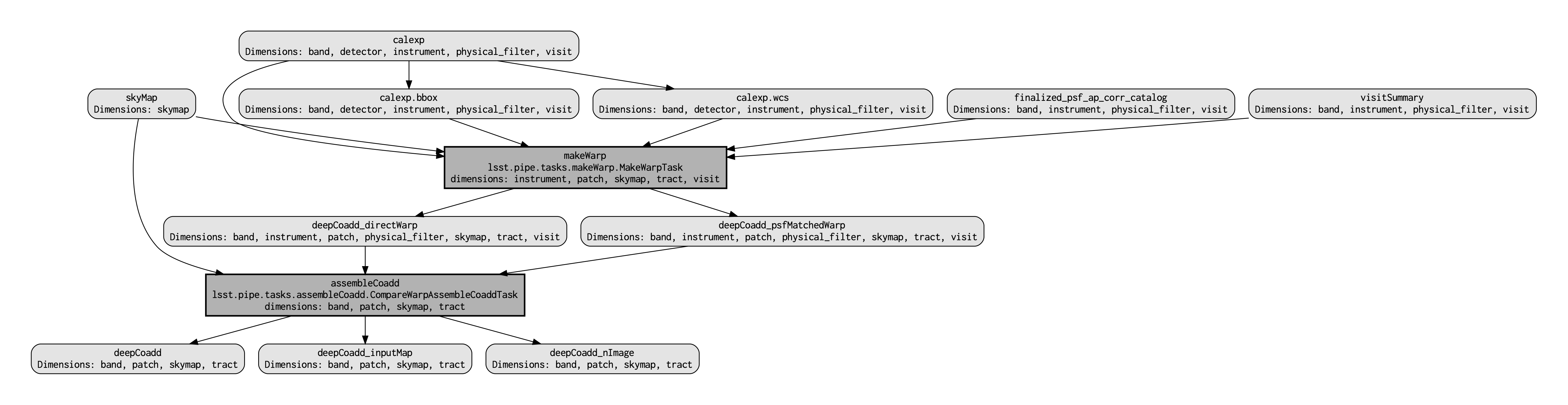
Here are some pointers on interpreting the QuantumGraph visualization:
Light gray rectangles with rounded corners represent data, whereas darker gray rectangles with sharp corners represent pipeline Tasks.
The arrows connecting the data and Tasks illustrate the data processing flow.
The data processing starts at the top, with the
calexpcalibrated single-exposure images (also known as Processed Visit Images; PVIs).The
makeWarpTask is applied to generate reprojected “warp” images from the various inputcalexpimages, and finally theassembleCoaddTask combines the warps intodeepCoaddcoadded products (light gray boxes along the bottom row).
Optional: Try running the following pipetask build command to generate the QuantumGraph visualization of the custom coadd processing:
pipetask build \
-p $DRP_PIPE_DIR/pipelines/LSSTCam-imSim/DRP-test-med-1.yaml#makeWarp,assembleCoadd \
--pipeline-dot pipeline.dot; \
dot pipeline.dot -Tpdf > makeWarpAssembleCoadd.pdf
This command executes very fast (roughly 5 seconds), again because it is not performing any search through the DP0.2 data set for e.g., input exposures. The pipeline.dot output is essentially an intermediate temporary file which you may wish to delete. The PDF you make (shown below) can be opened by double clicking on its file name in the JupyterHub file browser.
Step 4. Deploy your custom coaddition processing
As you might guess, the custom coadd processing is run via the pipetask run command. Because this processing takes longer than prior steps, it’s worth adding a little bit of “infrastructure” around your pipetask run command to perform logging and timing.
4.1. Set up for logging
First, let’s start by making a directory into which you’ll send the log file of the coaddition processing:
export LOGDIR=logs
mkdir $LOGDIR
Now you have a directory called logs into which you can save the pipeline outputs printed when creating your custom coadds.
4.2. The final custom coaddition commands
Now the a directory for output logs is in place, let’s also print out the processing’s start time at the very beginning and the time of completion at the very end, in both cases using the Linux date command. This will keep a record of how long your custom coadd processing took end-to-end. Send the date printouts both to the terminal and to the log file using the Linux tee command. Putting everything all together, the final commands to generate your custom coadds are:
LOGFILE=$LOGDIR/makeWarpAssembleCoadd-logfile.log; \
date | tee $LOGFILE; \
pipetask --long-log --log-file $LOGFILE run --register-dataset-types \
-b dp02 \
-i 2.2i/runs/DP0.2 \
-o u/$USER/custom_coadd_window1_cl00 \
-p $DRP_PIPE_DIR/pipelines/LSSTCam-imSim/DRP-test-med-1.yaml#makeWarp,assembleCoadd \
-c makeWarp:doApplyFinalizedPsf=False \
-c makeWarp:connections.visitSummary="visitSummary" \
-d "tract = 4431 AND patch = 17 AND visit in (919515,924057,924085,924086,929477,930353) AND skymap = 'DC2'"; \
date | tee -a $LOGFILE
Optional: For users familiar with using shell scripts, you can save the above commands to a shell script file and then launch that shell script. You could name the shell script file, for instance, dp02_custom_coadd_1patch.sh.
If you are not familiar with shell scripts, you can simply copy and paste the above commands into the terminal and hit the “return” key. The above commands take 30-35 minutes to run from start to finish. For brevity, the full output of executing the above pipetask run script is provided on a separate page.
The last line (before the timestamp printout) says “Executed 7 quanta successfully, 0 failed and 0 remain out of total 7 quanta”. So that means every subcomponent of this custom coadd processing was successful.
Step 5. Source detection, deblending, and measurement on your custom coadd
The following material corresponds to (a subset of) that contained in DP0.2 tutorial notebook 9b “Detect and Measure Sources in a Custom Coadded Image”, rather than DP0.2 tutorial notebook 9a.
5.1. The QuantumGraph for detection, deblending, and measurement
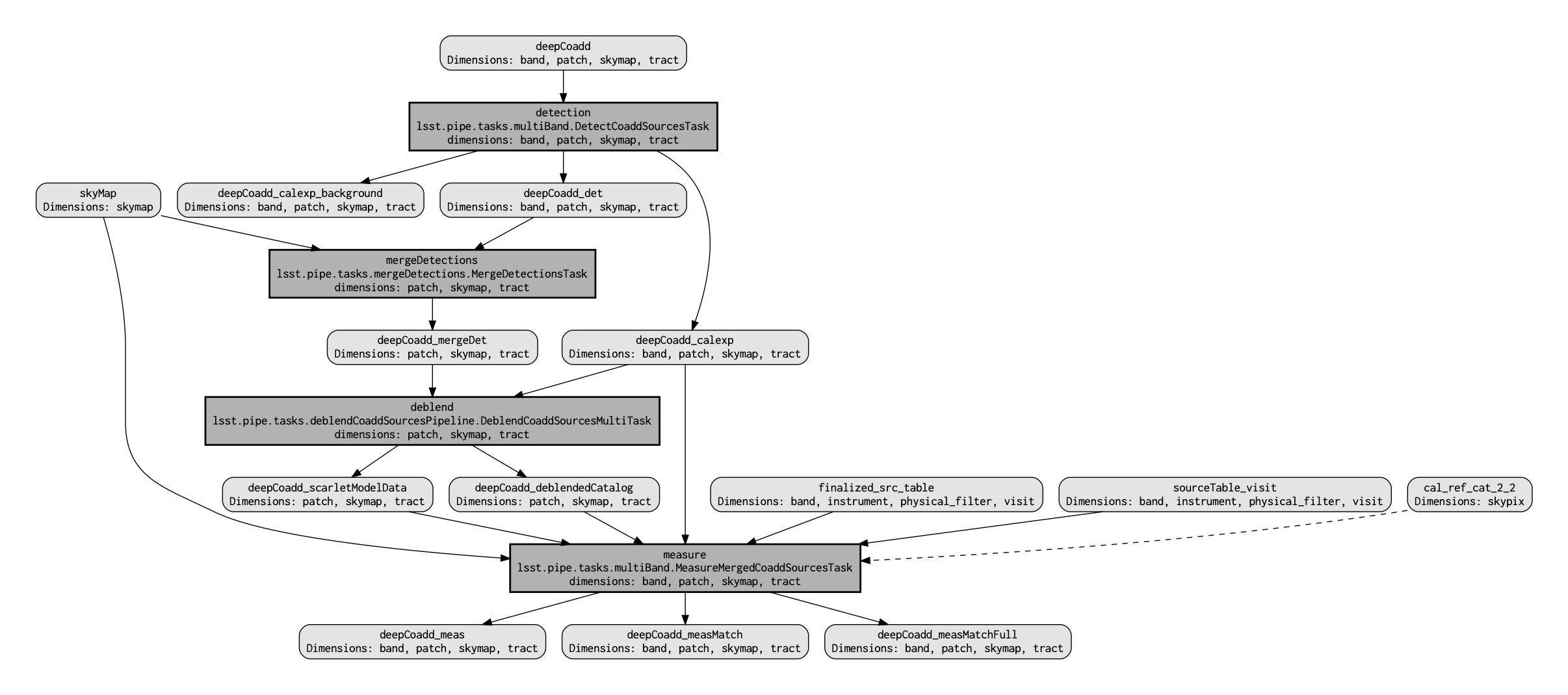
As with building the custom coadd, start by visualizing the workflow that will be followed during source detection, deblending and measurement using its QuantumGraph. Here’s what the QuantumGraph visualization looks like this time:
Optional: Try running the pipetask build command to create the above QuantumGraph visualization:
pipetask build \
-p $DRP_PIPE_DIR/pipelines/LSSTCam-imSim/DRP-test-med-1.yaml#detection,mergeDetections,deblend,measure \
--pipeline-dot pipeline.dot; \
dot pipeline.dot -Tpdf > detectionMergeDetectionsDeblendMeasure.pdf
As before, the pipeline.dot output is an intermediate temporary file which you may wish to delete.
This QuantumGraph visualization command is structurally the same as the command shown previously (and optionally executed) in Section 3.2 of this command line tutorial. A few notes on this command:
This
QuantumGraphvisualization command for source detection, deblending, and measurement uses the same pipeline definition YAML file as you have all throughout this command line tutorial. However, even though the URI passed topipetask buildhere includes the same YAML file name, the pipeline steps enumerated after the#symbol are different. In this case, the specific list of Data Release Production (DRP) steps to be included isdetection,mergeDetections,deblend,measure.The step labeled
detectionruns the actual source detection.The step labeled
mergeDetectionsis required in order for downstream steps to be able to use the results of thedetectionstep.The step labeled
deblendperforms deblending using the (merged) results of the detection step and the i-band custom coadd itself.Lastly, the step labeled
measurecomputes useful quantities, such as the photometric fluxes, given the deblended list of sources.
The detectionMergeDetectionsDeblendMeasure-DRP.pdf visualization generated by the above pipetask build command looks as follows:
5.2. Deploy detection, deblending, and measurement
To perform source detection, deblending, and measurement on your custom i-band coadd rather than only visualizing the QuantumGraph, execute the following:
LOGFILE=$LOGDIR/detectionMergeDetectionsDeblendMeasure.log
pipetask --long-log --log-file $LOGFILE run \
-b dp02 \
-i u/$USER/custom_coadd_window1_cl00 \
-o u/$USER/custom_coadd_window1_cl00_det \
-c detection:detection.thresholdValue=10 \
-c detection:detection.thresholdType="stdev" \
-c deblend:multibandDeblend.maxIter=20 \
-c measure:doPropagateFlags=False \
-p $DRP_PIPE_DIR/pipelines/LSSTCam-imSim/DRP-test-med-1.yaml#detection,mergeDetections,deblend,measure \
-d "tract = 4431 AND patch = 17 AND band = 'i' AND skymap = 'DC2'"
This command takes approximately 10-12 minutes to run.
Note a few things about this command:
The URI specified here via the
-pargument is the same as used when visualizing the correspondingQuantumGraph.The same
-b dp02Butler repository is specified as was used for custom coaddition.The
-iinput argument now points to what was previously the output-oargument for custom coaddition – that is, the output of custom coaddition has now become the input for running source detection/measurement on the custom coadd.The
-oargument specifies a collection that’s different from the input collection. This is a recommended best practice for the sake of Butler’s provenance tracking. Also, for the sake of provenance, make sure that the-ooutput collection is a new collection rather than an existing one.The first two
-cconfiguration overrides are needed to parallel the configuration overrides used in notebook tutorial 9b, specifically setting the detection threshold to 10 sigma.The
-c deblend:multibandDeblend.maxIter=20configuration override sets the maximum deblending iterations to a lower value than its default, which is a recommended mechanism for speeding up the processing.The
-c measure:doPropagateFlags=Falseconfiguration override is set because this processing does not need to propagate flag information about which sources were used for PSF construction.
The full output of this section’s pipetask run command is shown on a separate page for brevity.
Optional exercises for the learner
Proceed to DP0.2 tutorial notebook 9b. Option 1: use the custom coadd outputs from Step 4 of this command line tutorial as the input for running the entirety of DP0.2 tutorial 9b. Option 2: use the source detection outputs from Step 5 of this command line tutorial as an input for Step 3 of DP0.2 tutorial notebook 9b.
Try modifying other configuration parameters for the
makeWarpand/orassembleCoaddtasks via thepipetask-cargument syntax.Try using the same two configuration parameter modifications as did this tutorial, but implementing them via a separate configuration (
.py) file, rather than via thepipetask-cargument (hint: to do this, you’d use the-Cargument forpipetask).Run the
pipetask qgraphcommand from section 3.1, but with the final line--show graphremoved. This still takes roughly 15 minutes, but prints out a much more concise summary listing only the total number of quanta to be executed, which should be 7.