Introduction to the RSP Portal Aspect
Log in to the Portal Aspect by clicking on the “Portal” panel of the main landing page at data.lsst.cloud.
New for DP0.2! Image Search (ObsTAP)
Last verified to run: in the original version November 2023; updates to reflect the new UI starting May 16 2024
The Portal’s user interface
The Rubin Science Platform Portal Aspect has a variety of search functions that can access DP0.2 Images, DP0.2 Catalogs, and DP0.3 (Solar System only) Catalogs. Once you log in to the Rubin Science Platform and select “Portal aspect” you will see the multiple tabs on top. Clicking on the respective tab will allow you to work with any of those image / catalog repositories. Within each tab, there are multiple types of queries that can be performed. Within those three choices above, there is the ability to use “UI assisted” searching or ADQL queries. Each of these options has a different user interface, covered in the sections below. The rightmost tab allows you to upload your own images or tables, but its use is more advanced and will not be covered here. The leftmost tab marked as “Results” will contain the result of your query. If you execute several queries, the results of those queries will appeas as separate sub-tabs in the “Results” tab.
In this Introduction, we will focus on the DP0.2 catalogs and images, but we note that the functionality described here also applies to the DP0.3 catalogs. Note that DP0.3 simulations contain only catalogs (no images).
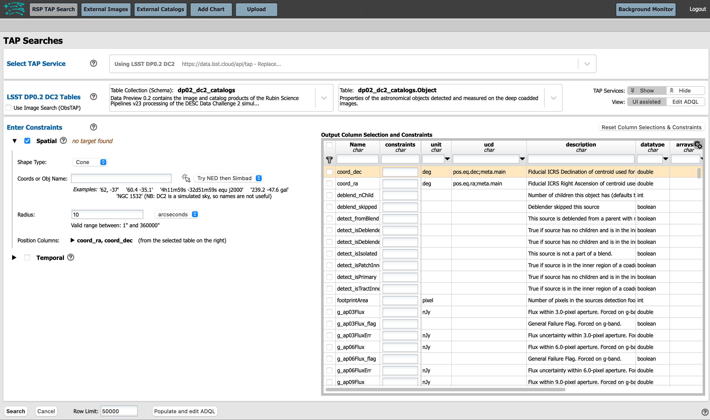
The default view of the Portal’s user interface for UI assisted queries.
Try it: Mouse-over text to view pop-up boxes with more detailed descriptions throughout the Portal interface. Click on any “settings” icons you see (single gear) to explore options. The Portal is a very powerful user interface with far more options than are covered in the introduction below.
Sample query of one of the the DP0.2 catalogs
Select Query Type The default landing page will be the one for “DP0.2 Catalogs” and we will begin with DP0.2 to get you started. There, you have two types of queries: “UI Assisted” (amounting to single-table queries - default), or “ADQL Queries”.
Once you selected the choice of data repository, you can select either to conduct your query. Each of these options has a different user interface, covered in the sections below.
UI assisted (Single Table)
The default query type, and default user interface, is for “UI assisted” queries.
Select Table: Once you click on the “DP0.2 Catalogs” tab, you can choose the table to work with by clicking the “up-down” arrow to show the available tables. The default table in the right drop-down menu is the Object table, and we will use this table for this introduction. See the DP0.2 Data Products Definition Document (DPDD) for table descriptions and schema. Notice how the table view at lower-right will automatically update to match the table selected by you (via clicking the “up-down” arrow).
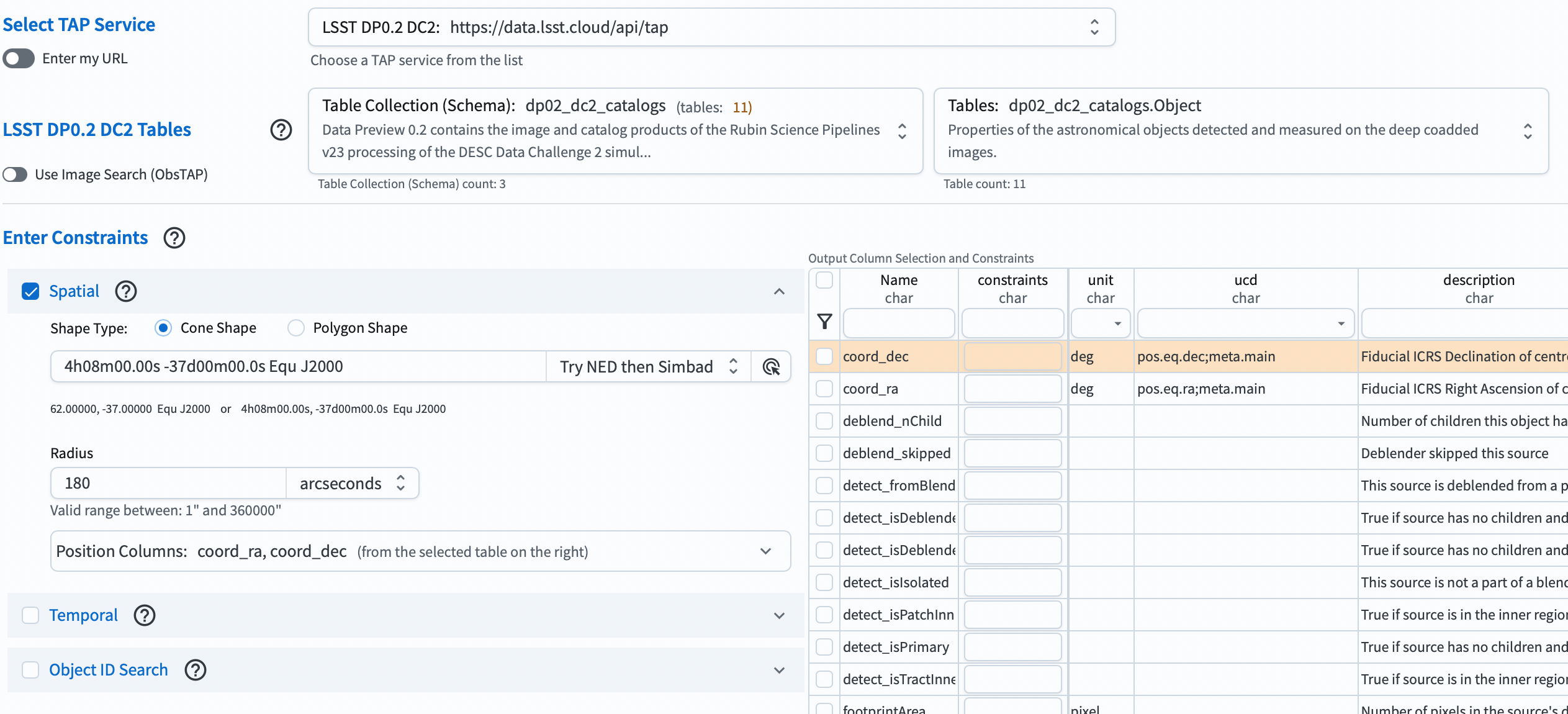
Enter Constraints: Check the box by “Spatial.” For “Spatial” constraints, choose the desired shape type for a spatial search (“Cone” or “Polygon”), and the appropriate instructions for the search terms will appear. For example, for cone search, “Coordinates or Object Name” and “Radius” of search need to be entered.
Keeping the search area small will keep query times short and return manageable subsets of objects as you learn.
It is recommended to start with 3 arcminutes.
Note that the central (RA, Dec) coordinates for DC2, in decimal degrees, are: 61.863 -35.790.
The longitude and latitude columns in “Position Columns” do automatically update to be the correct column names for right ascension and declination for the selected table. If a non-existent column name is entered, the box will highlight red in indication of the error.
The table view: The table to the right of “Enter Constraints” enables users to apply additional search constraints on the columns in the selected catalog table. Some tables have a lot of data columns. Search for desired data columns by entering terms (e.g., ra, Flux, or flag) in the boxes underneath “Name” and pressing “enter” in order to view data columns of interest to you. Entering, e.g. “ra” will return all rows containing “ra” in the name.
Use the checkboxes in the left-most column to select the data column names to be returned by the query. Use the funnel icon to filter the columns, and only view selected data column names. Use the “constraints” column to specify query parameters and only retrieve data which meets those constraints.
Remove filters and reset the table view at any time using the “Reset Column Selections & Constraints” button above the upper-right corner of the table.
ADQL conversions: If desired, convert UI assisted table view queries to “ADQL Queries” using the “Populate and edit ADQL” button at the bottom of the page. This can enable entering more complex constraints that cannot be expressed against individual columns. This will switch the user interface to the “Edit ADQL” view. The searches using ADQL are described in more detail in the section “Edit ADQL (advanced)” below.
Row limit: The “Row Limit” in the bottom of the page can be changed to apply an upper bound to the number of rows returned. The Portal can work effectively with datasets with millions of rows. However, when learning or testing queries, it is advisable to limit the number of rows (e.g., 10000 rows is useful for testing).
Note: Because of the implementation of the Rubin Observatory “QServ” database, it is not recommended to use the row limit alone in order to get a “sampling” of data. Queries with only a row limit can run for much longer than one might intuitively expect; applying a spatial constraint is likely to return a result more quickly.
Example UI assisted query: The image below presents an example of how to search the DP0.2 Object catalog using a 3 arcminute cone near the DC2’s central coordinates, returning only the five data columns “coord_ra”, “coord_dec”, and “g” “r” and “i_calibFlux”, and imposing the contraints that the flux must be between 20 and 1000 nanojansky (i.e., between 24th and 28th magnitude).
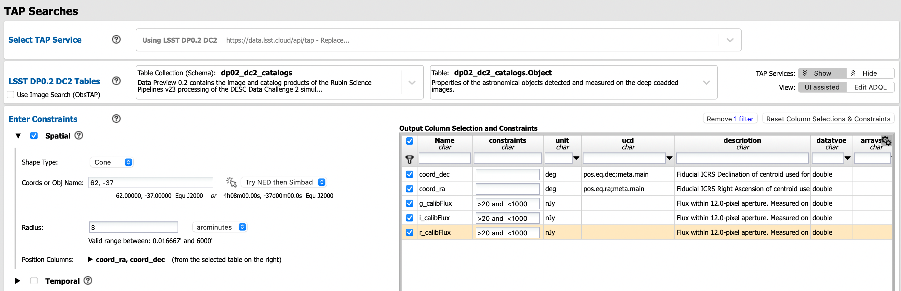
An example query of the DC2 Object catalog.
Search: Press the search button at lower left when ready to execute. The search might take a few moments.

This will show while the search is executing.
Cancel: It is possible to cancel a query while it is executing by clicking the “Cancel” button.
Results view: The search results will populate the “Results” view, as shown in the figure below. The display layout is controlled by the “hamburger” button (three horizontal lines) at upper left. You can change the layout by clicking on this icon and then on the “Results Layout” tab. The screenshot below uses the “Coverage Charts Tables” choice with a sky image at upper left. The color-composite image shows the relevant DC2 simulated sky region. A default “active chart” of the sky coordinates appears at upper right, and the table of results along the bottom. Note that by default, the “active chart” displays the two leftmost columns in the table against each other.
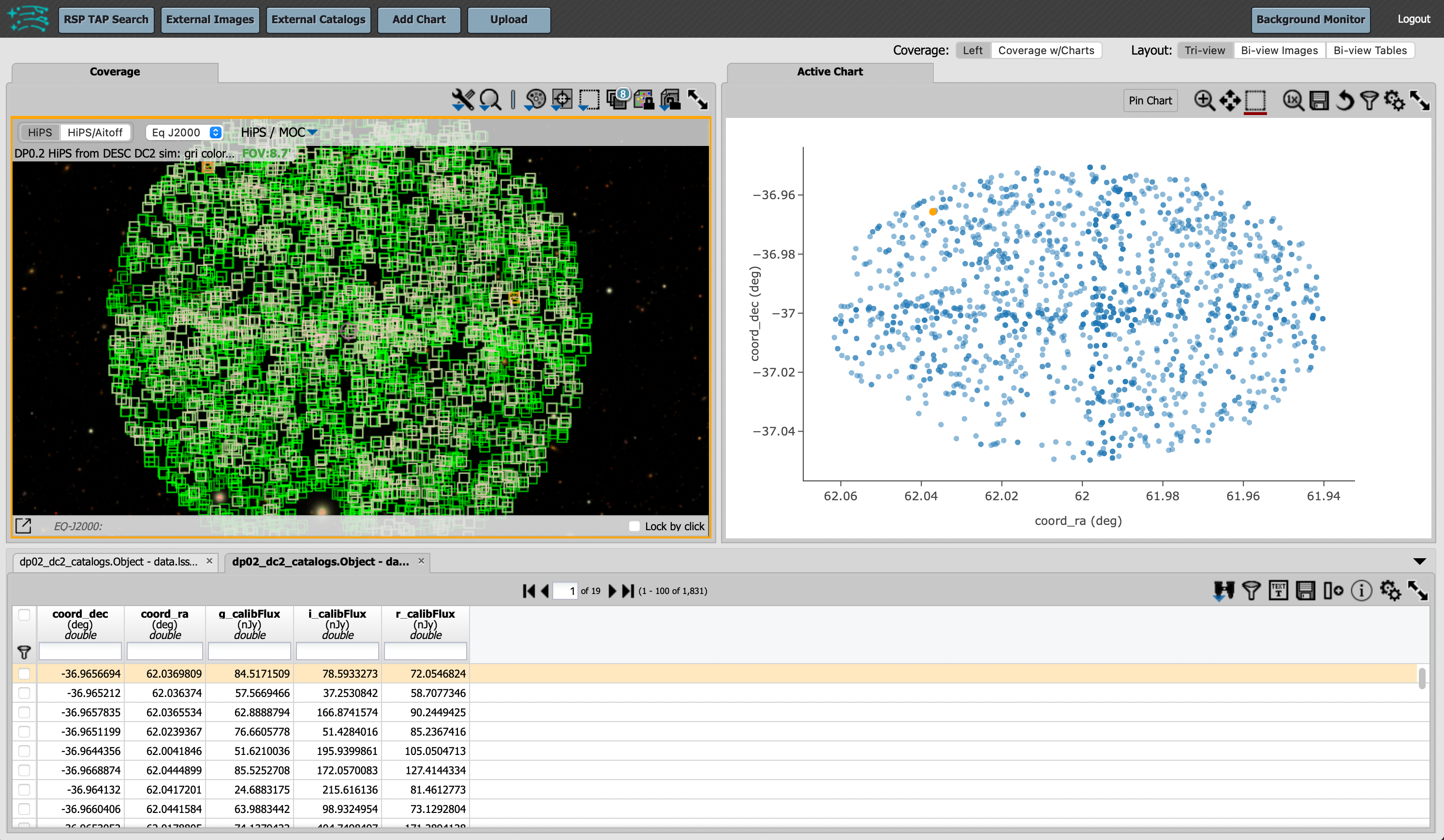
The default view of the search results.
Multiple queries and results: From the results view page (see figure above), if you click on the “DP0.2 Catalogs” tab on top, you can go back to the query page. There, you can execute another query by entering constraints and clicking “Search”. (Click “Cancel” on the TAP search page to return to the results view without executing a new query).
The new query’s results will appear as a new tab in the table of the results view page. In the image above, you can see that this has been done, because the results view table has three tabs. Switching between table tabs will also cause the sky image and active chart to switch to show the selected query results. Delete the results for a given query by clicking on the x in the table tab.
Manipulating the plotted data and converting fluxes to magnitudes: To manipulate the plotted data, select the single gear “settings” icon above the active chart and a pop-up window will open (see the next figure). To create a color-magnitude diagram from the fluxes, for DP0.2 it is necessary to apply the standard conversion from nanojansky to AB magnitude in the X and Y boxes as, e.g., “-2.5 * log10(g_calibFlux) + 31.4”. In the future, magnitudes will be available.
Add a chart title and label the axes, choose a point color, and click “Apply” and then “Close”.
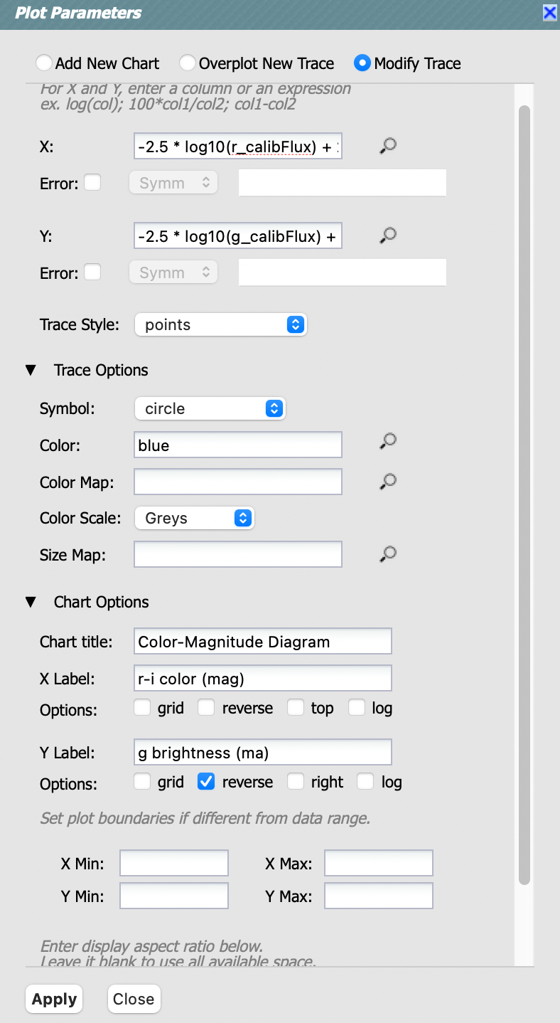
The plot settings pop-up window.
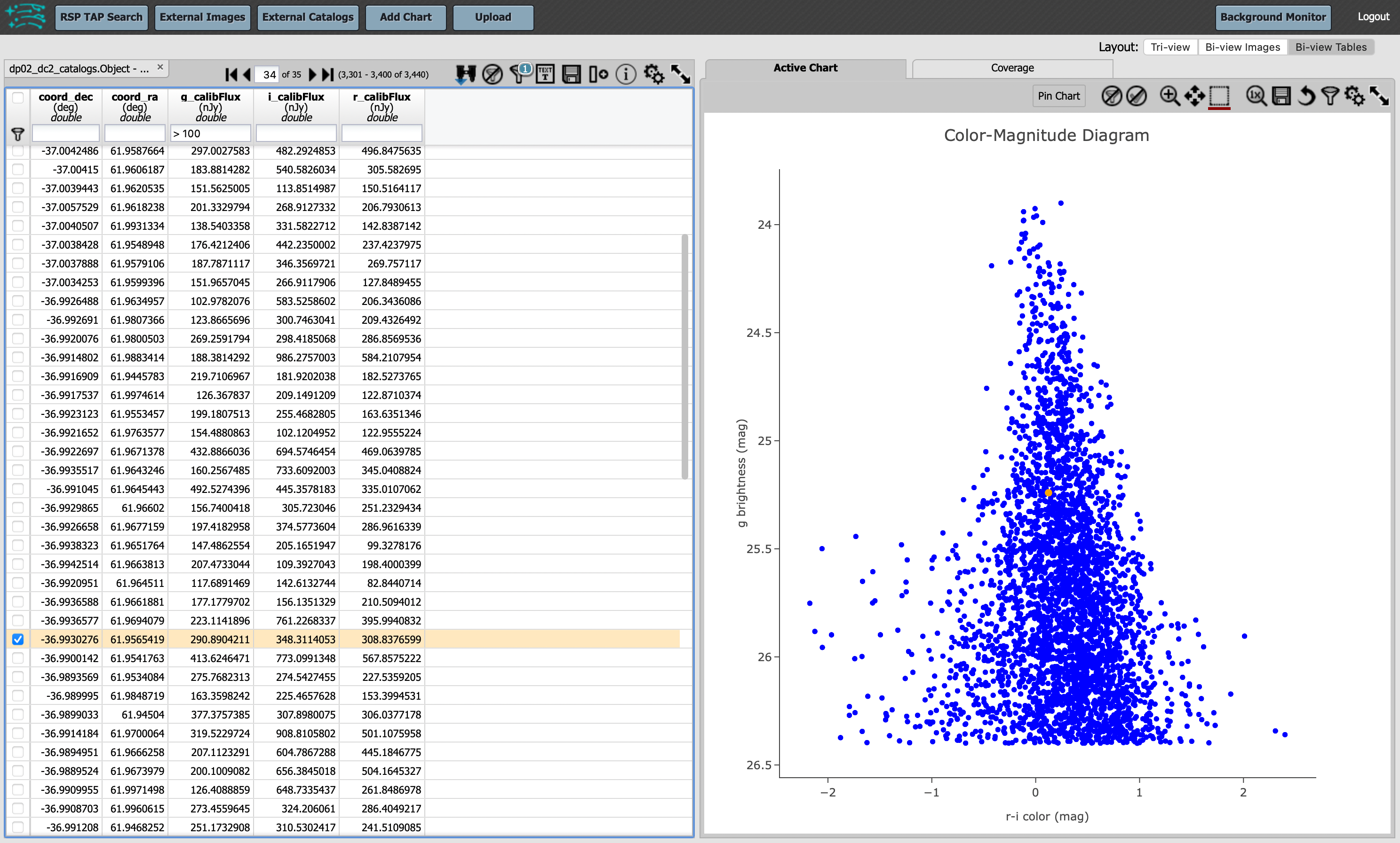
At this point, additional cuts can be applied to the table data being plotted. In the figure below, the g-band flux is limited to >100 (via the constraint entered in the header of the column “g_calibFlux”), and this imposes a sharp cutoff in the y-axis values at 26.4 mag. Convert the plot to “Tables Coverage Charts” using the “hamburger” menu at upper left and select only the “Active Chart” tab. Click on any row in the table on the left, and notice how the corresponding plot point for the selected row in the table is differently colored, and that hovering the mouse over the plotted data will show the x- and y-values in a pop-up window.
Learn more. See also Portal tutorials for additional demonstrations of how to use the Portal’s UI assisted Query.
Edit ADQL (advanced)
ADQL is the Astronomical Data Query Language. The language is used by the IVOA to represent astronomy queries posted to Virtual Observatory (VO) services, such as the Rubin LSST TAP service. ADQL is based on the Structured Query Language (SQL).
Selecting “Edit ADQL” will change the user interface to display an empty box where users can supply their query statement. Scrolling down in that interface will show several examples.
Turn a UI assisted (i.e., single table) query into ADQL. At any point while assembling a query using the UI assisted query interface described above, clicking on “Populate and edit ADQL” at the bottom of the page will transform the query into ADQL. Note that any changes then made to the ADQL are not propogated back to the UI assisted query constraints.
Converting fluxes to magnitudes is much easier with the ADQL interface by using the scisql_nanojanskyToAbMag() functionality as demonstrated below.
Query the TAP schema. Information about the LSST TAP schema can be obtained via ADQL queries. For example, to get the detailed list of columns available in the “Object” table, their associated units and descriptions:
SELECT tap_schema.columns.column_name, tap_schema.columns.unit,
tap_schema.columns.description
FROM tap_schema.columns
WHERE tap_schema.columns.table_name = 'dp02_dc2_catalogs.Object'
Query the Object table, as done with the UI assisted query interface above, with the following ADQL:
SELECT coord_dec,coord_ra,g_calibFlux,i_calibFlux,r_calibFlux
FROM dp02_dc2_catalogs.Object
WHERE CONTAINS(POINT('ICRS', coord_ra, coord_dec),CIRCLE('ICRS', 62, -37, 0.05))=1
AND (g_calibFlux >20 AND g_calibFlux <1000
AND i_calibFlux >20 AND i_calibFlux <1000
AND r_calibFlux >20 AND r_calibFlux <1000)
Type the above query into the ADQL Query block and click on the “Search” button in the bottom-left corner to execute. Remember to set the “Row Limit” to be a small number, such as 10000, when testing queries. The search results will populate the same Results View, as shown above using the UI assisted Query interface.
To do the same query with magnitudes:
SELECT coord_dec, coord_ra,
scisql_nanojanskyToAbMag(g_calibFlux) AS g_calibMag,
scisql_nanojanskyToAbMag(i_calibFlux) AS r_calibMag,
scisql_nanojanskyToAbMag(r_calibFlux) AS i_calibMag
FROM dp02_dc2_catalogs.Object
WHERE CONTAINS(POINT('ICRS', coord_ra, coord_dec),
CIRCLE('ICRS', 62, -37, 0.05))=1
AND g_calibFlux BETWEEN 20 AND 1000
AND r_calibFlux BETWEEN 20 AND 1000
AND i_calibFlux BETWEEN 20 AND 1000
Joining two or more tables. It is often desirable to access data stored in more than just one table. This is possible to do using a JOIN clause to combine rows from two or more tables. In the example below, the Source and CcdVisit table are joined in order to obtain the date and seeing from the CcdVisit table. Any two tables can be joined so long as they have an index in common.
SELECT src.ccdVisitId, src.extendedness, src.band,
scisql_nanojanskyToAbMag(src.psfFlux) AS psfAbMag,
cv.obsStartMJD, cv.seeing
FROM dp02_dc2_catalogs.Source AS src
JOIN dp02_dc2_catalogs.CcdVisit AS cv
ON src.ccdVisitId = cv.ccdVisitId
WHERE CONTAINS(POINT('ICRS', coord_ra, coord_dec),
CIRCLE('ICRS', 62.0, -37, 1)) = 1
AND src.band = 'i' AND src.extendedness = 0 AND src.psfFlux > 10000
AND cv.obsStartMJD > 60925 AND cv.obsStartMJD < 60955
Learn More. See also Portal tutorials for additional demonstrations of how to use the Portal’s ADQL functionality.
Image Search (ObsTAP)
You can perform image searches by clicking in the “DP0.2 Images” tab on top of the screen. This functionality has many new features – not just new for DP0.2, but new to the Firefly interface, and DP0 users are among the first to use them. Clicking on that tab will change the user interface to display query constraint options that are specific to the image data, as described below.
For more information about the image types available in the DP0.2 data set, see the DP0.2 Data Products Definition Document (DPDD).
Enter Constraints
Under “Observation Type and Source”, the IVOA standard options for “Calibration Level” (0, 1, 2, 3, or 4) are provided. For DP0.2, “1” is the raw (unprocessed) images, “2” is the processed visit images (PVIs; the calibrated single-epoch images also called calexps), and “3” are the derived image data such as difference images and deep coadds.
The “Data Product Type” should be left as “Image”, and the “Instrument Name”, “Collection”, and “Data Product Subtype” can all be left blank.
Under “Location”, only “Observation boundary contains point” was implemented at the time this documentation was written.
Recall that the central (RA, Dec) coordinates for the DC2 simulated sky region are 61.863 -35.790.
Under “Timing”, users can specify a range of the time of observation (this is only relevant for PVIs/calexps) and/or exposure duration.
Under “Spectral Coverage”, users can provide a wavelength in, e.g., nanometers as a means of specifying the image band.
Output Column Selection and Constraints
The default is for all columns to be selected (i.e., have blue checks in the leftmost column). It is recommended to always return all metadata because the Portal requires some columns in order for the some of the “Results” view functionality to work.
Example (PVIs/calexps)
The screenshot below shows an example query for all PVIs (calexps) that overlap the central coordinates of DC2, which were obtained with a modified Julian date between 60000 and 60500.
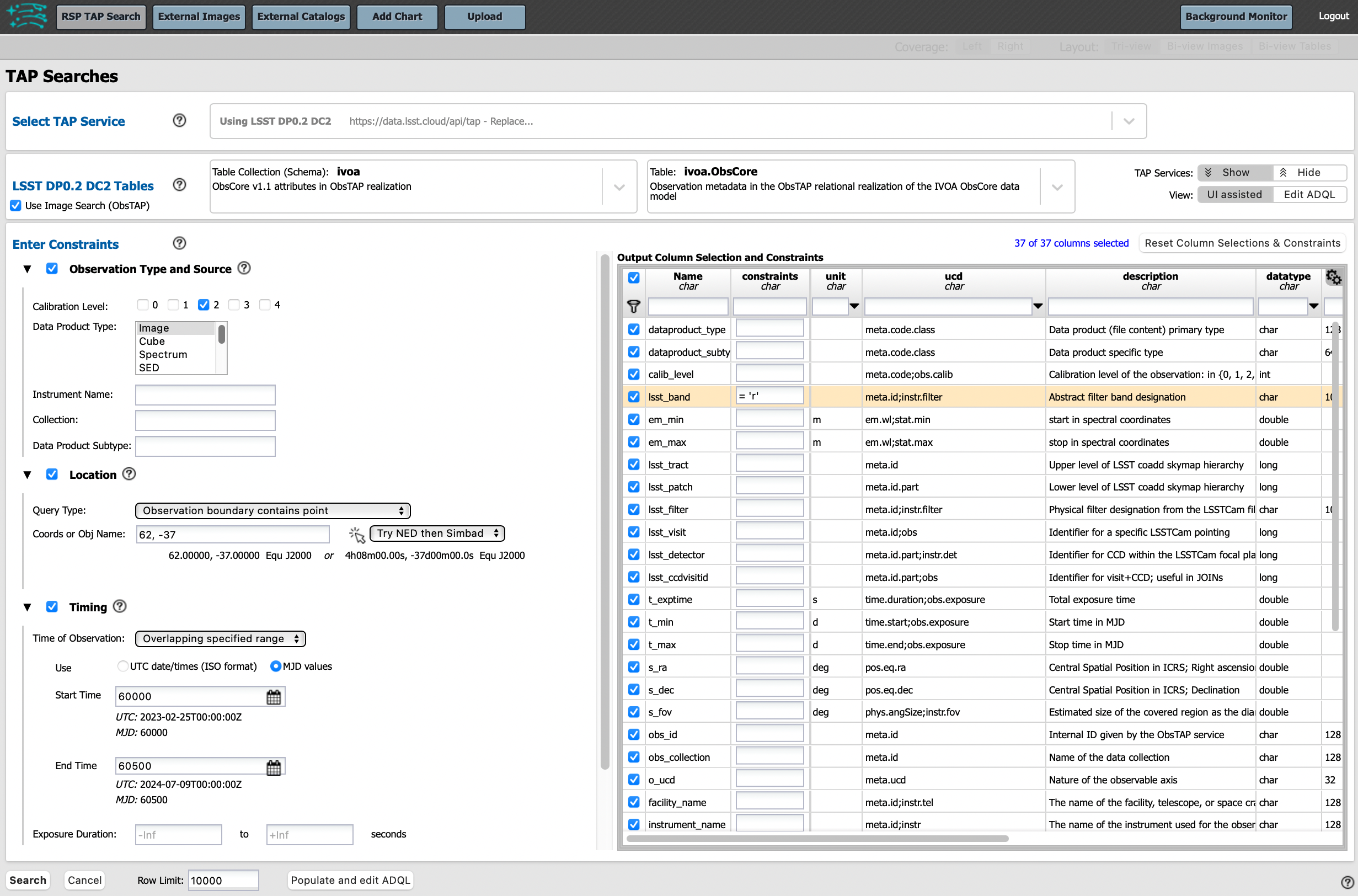
Click on the “Search” button. Note that this search retrieves observations in all filters.
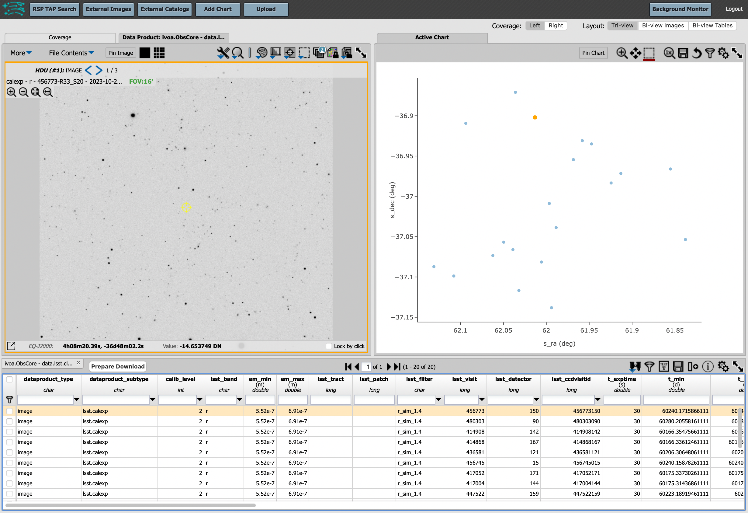
Results View
The default results appear in the tri-view format, with the image at upper left, an Active Chart plot at upper right, and the table of metadata below. The first row of the table is highlighted by default, with the corresponding image showing at upper left. The Active Chart plot default is RA versus Declination, with the location of the highlighted table row shown in orange and the rest in blue. You can restrict the retrieved images to be only those in the ‘r’ filter by clicking the down-arrow below the table column heading “lsst_band” and selecting “r” from the drop-down menu.
Manipulating the Active Chart plot is the same process as shown for the UI assisted (Single Table) results: click on the “settings” icon (single gear) in the upper right corner to change the column data being plotted, alter the plot style, add axes labels, etc.
Interacting with the images begins with just hovering the mouse over the sky image and noting the RA, Dec, and pixel value appear at the bottom. Use the magnifying glass icons in the upper left corner to zoom in and out. You might need to hover over the image for these magnifying glasses to appear on the upper left. Click and drag the image to pan. Above the magnifying glass icons, use the back and forth arrows to navigate between HDU (header data units) 1, 2, and 3: the image, mask, and variance data. Click on another row in the table, to display an image of a different part of the sky. At upper left, click on the “hamburger” menu, and in the “Results Layout” tab, select “Tables / Coverage Images Charts” option. On the right-hand side, select “Data Product: ivoa.ObsCore” tab. This will result in the table and the sky image side-by-side.
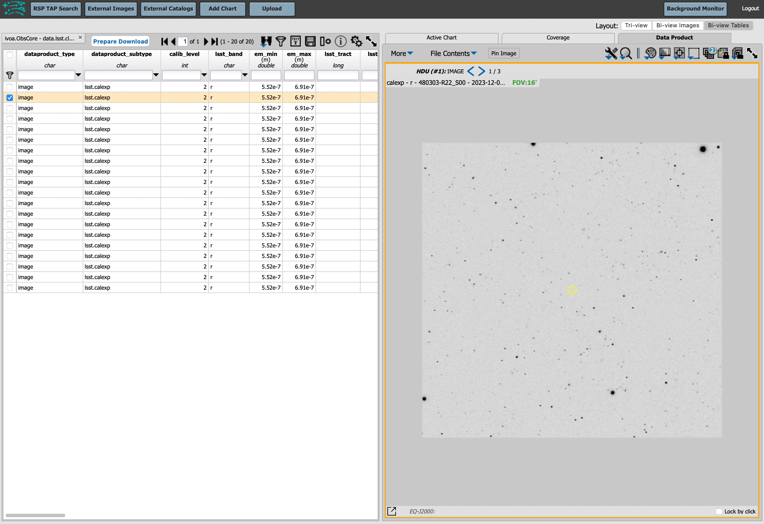
Image tools: There are many tools available for users, the following demonstrates use of just one. First, zoom in on a bright star in one of the images. Select the “tools” icon (wrench and hammer), and from the pop-up window choose to “Extract” using a line. Draw a line on the image across the star to extract the pixel values and show an approximate shape of the point-spread function (PSF) for the star. The plot reveals that this particular star is saturated. Click on “Pin Chart/Table” to add a table of pixel data as a new tab in the left half of the view (the “Tables” side) as well as the PSF profile plot as a new tab next to Active Chart plot (the tab is marked as “Pinned Charts”). To make the line go away, click on the “layers” icon (the one for which the hover-over text reads: “Manipulate overlay display…”) and in the pop-up window, next to “Extract Line 1 - HDU#1”, click on “x” by the “Extract Line Tool” row.
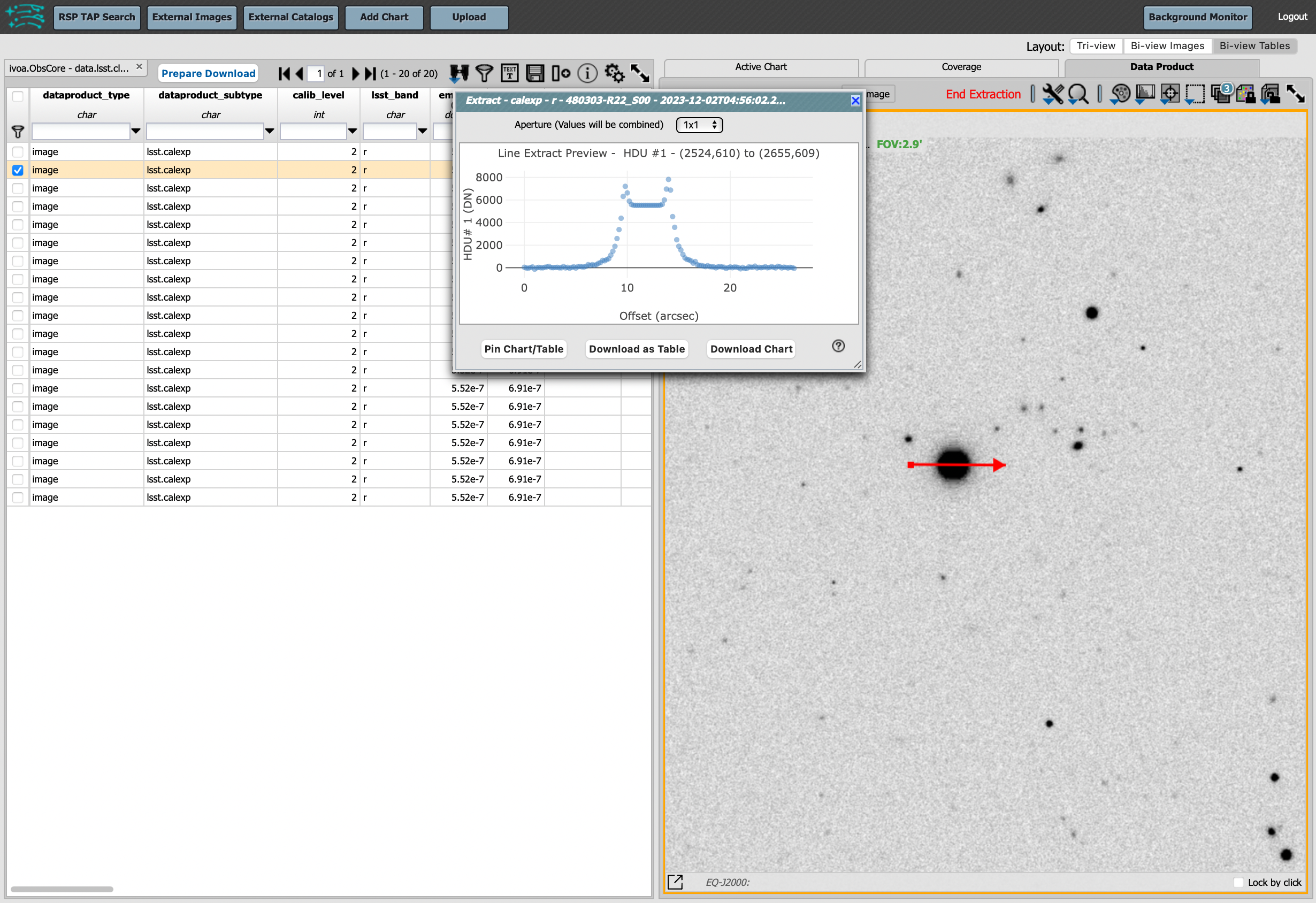
Image grid display: Close all pop-up windows. Above the image use the grid icon (hover-over text “Tile all images in the search result table”) to show up to eight of the images side-by-side. Notice that it is possible to pan and zoom in each of these grid windows.
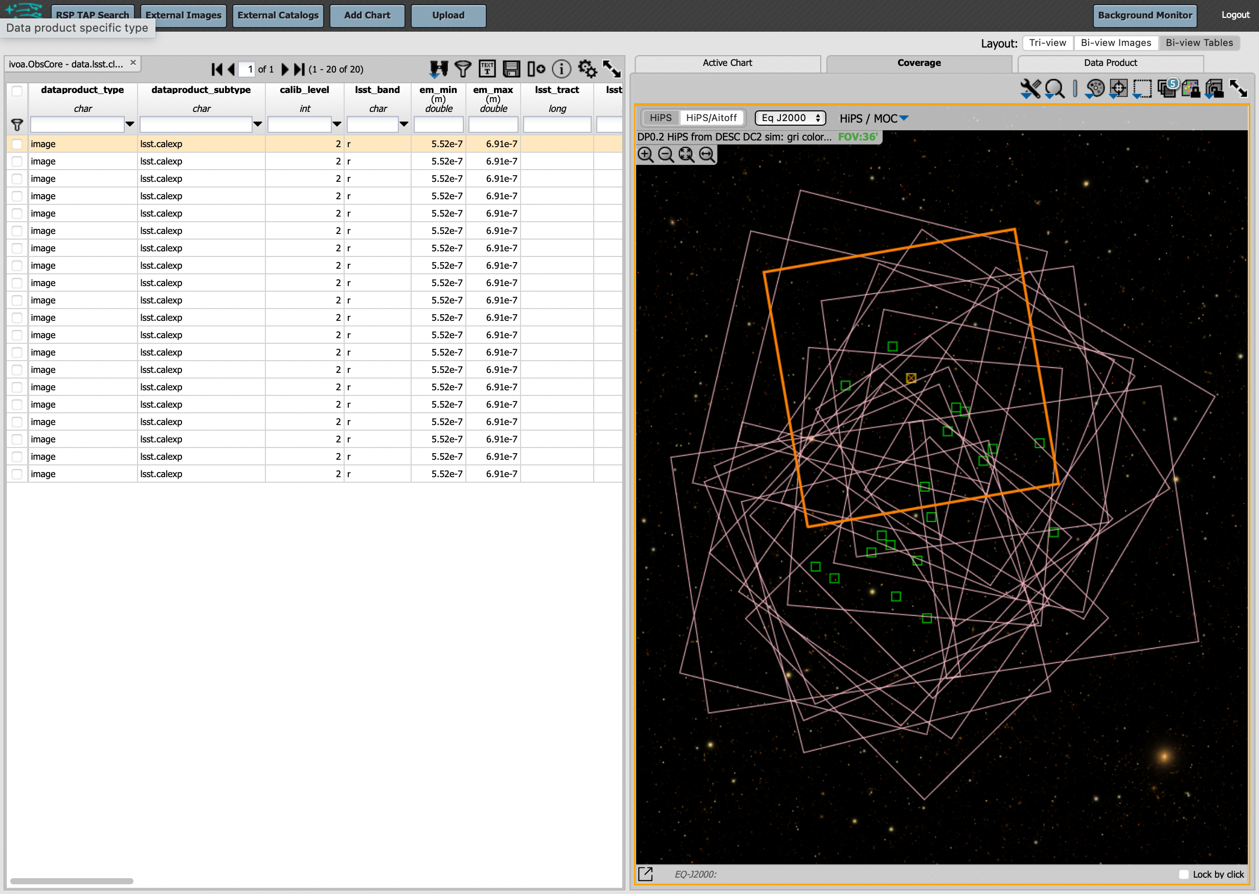
Coverage window: Above the image, notice that the default tab view is “Data Product: ivoa.obs.core”, and instead click on “Coverage”. The bounding boxes of all images listed in the table are shown, with the image in the selected row highlighted. The color-composite background shows the relevant DC2 simulated sky region.
Learn More. See also Portal tutorials for a tutorial using additional image types and more of the Portal’s image-related functionality.
Public URL API for the Portal
The public Uniform Resource Locator (URL) Application Programming Interface (API) provides direct access to specific resources via a publicly accessible URL; however, an RSP login is still required.
One application is to construct URLs for your ADQL queries, enabling you to share these links with collaborators for efficient communication or save them for future reuse, avoiding the need to repopulate the ADQL edit box each time. Use the following examples as a guide to construct your own.
1. Exploring the Object table
To learn about the contents of a tableto, retrieve the first 100 rows of the Object table using the SELECT TOP statement.
SELECT TOP 100 * FROM dp02_dc2_catalogs.Object
Corresponding URL API:
https://data.lsst.cloud/portal/app/?api=tap&service=https://data.lsst.cloud/api/tap&adql=SELECT%20TOP%20100%20*%20FROM%20dp02_dc2_catalogs.Object&execute=true
2. Populate the ``UI-assisted’’ page for a cone search
The URL below populates the “UI-assisted” page to perform a cone search on the Object catalog using a radius of 0.05 degrees centered at (RA, Dec) = (62, -37).
URL API:
https://data.lsst.cloud/portal/app/?api=tap&service=https://data.lsst.cloud/api/tap&schema=dp02_dc2_catalogs&table=dp02_dc2_catalogs.Object&ra=62.0&dec=-37.0&sr=0.05d
3. Execute the cone search above
You can also perform this search by editing the ADQL query box and clicking the search button. Below is the ADQL query for the cone search, along with the URL API that executes the search directly.
SELECT coord_dec, coord_ra
FROM dp02_dc2_catalogs.Object
WHERE CONTAINS(POINT('ICRS', coord_ra, coord_dec),
CIRCLE('ICRS', 62, -37, 0.05)) = 1
Corresponding URL API:
https://data.lsst.cloud/portal/app/?api=tap&service=https://data.lsst.cloud/api/tap&adql=SELECT%20coord_dec,coord_ra%20FROM%20dp02_dc2_catalogs.Object%20WHERE%20CONTAINS(POINT('ICRS',coord_ra,coord_dec),CIRCLE('ICRS',62,-37,0.05))%3D1&execute=true
4. Search for coadded images
The URL below will directly perform a search for coadded images containing the specified coordinates above.
URL API:
https://data.lsst.cloud/portal/app/?api=tap&service=https://data.lsst.cloud/api/tap&schema=ivoa&table=ivoa.ObsCore&worldPt=62.0;-37.0;EQ_J2000&obsCoreSubType=lsst.deepCoadd_calexp&execute=true
5. Convert fluxes to magnitudes
The ADQL query below retrieves columns for the specified coordinates above, including the g-band AB magnitude and its error, converted from the g_calibFlux and g_calibFluxErr columns. The corresponding URL to execute the query directly is also provided.
SELECT coord_dec, coord_ra,
scisql_nanojanskyToAbMag(g_calibFlux) AS g_calibMag,
scisql_nanojanskyToAbMagSigma(g_calibFlux, g_calibFluxErr) as g_calibMagErr
FROM dp02_dc2_catalogs.Object
WHERE CONTAINS(POINT('ICRS', coord_ra, coord_dec),
CIRCLE('ICRS', 62, -37, 0.05)) = 1
Corresponding URL API:
https://data.lsst.cloud/portal/app/?api=tap&service=https://data.lsst.cloud/api/tap&adql=SELECT%20coord_dec,%20coord_ra,%20scisql_nanojanskyToAbMag(g_calibFlux)%20AS%20g_calibMag,%20scisql_nanojanskyToAbMagSigma(g_calibFlux,%20g_calibFluxErr)%20AS%20g_calibMagErr%20FROM%20dp02_dc2_catalogs.Object%20WHERE%20CONTAINS(POINT('ICRS',%20coord_ra,%20coord_dec),%20CIRCLE('ICRS',%2062,%20-37,%200.05))%3D1&execute=true
6. Populate the ``Edit ADQL’’ page with a search for a specific object
The URL below populates the ``Edit ADQL’’ page to perform a search for a specific object with ObjectId=1651220174314974795.
URL API:
https://data.lsst.cloud/portal/app/?api=tap&service=https://data.lsst.cloud/api/tap&adql=select%20*%20from%20dp02_dc2_catalogs.Object%20where%20objectId=1651220174314974795
Note. Currently, using this API involves a degree of shared risk, as further modifications are anticipated prior to DP1 and the commencement of survey operations.