05. Making Multiband Lightcurves with Forced Photometry
RSP Aspect: Portal
Contact authors: Greg Madejski and Melissa Graham
Last verified to run: 2024-05-03
Targeted learning level: intermediate
Introduction:
In Portal Tutorial 02, a supernova lightcurve was plotted using the measurements in the DiaSource table,
but the DiaSource table only contains measurements when the supernova is detected with SNR > 5
in the difference image.
If your science goal requires lower-SNR measurements (e.g. including fluxes of a given object measured during all visits to its location,
for instance before and after a flare or explosion), then use the forced photometry in the ForcedSourceOnDiaObject table instead.
This tutorial demonstrates how to create a forced photometry lightcurve for the same supernova used in
Portal Tutorial 02, which has a DiaObjectId of 1252220598734556212.
Step 1. Plot a single-band lightcurve
This first step is a repeat of Portal Tutorial 02, and can be skipped.
1.1. Log in to the Portal Aspect of the Rubin Science Platform, and select “DP0.2 Catalogs” tab.
1.2. At upper right on the main Portal user interface, click “Edit ADQL” to switch to the ADQL query view. (In the figure below, see the red arrow.) Clear the content of the ADQL query box, if it is not empty.
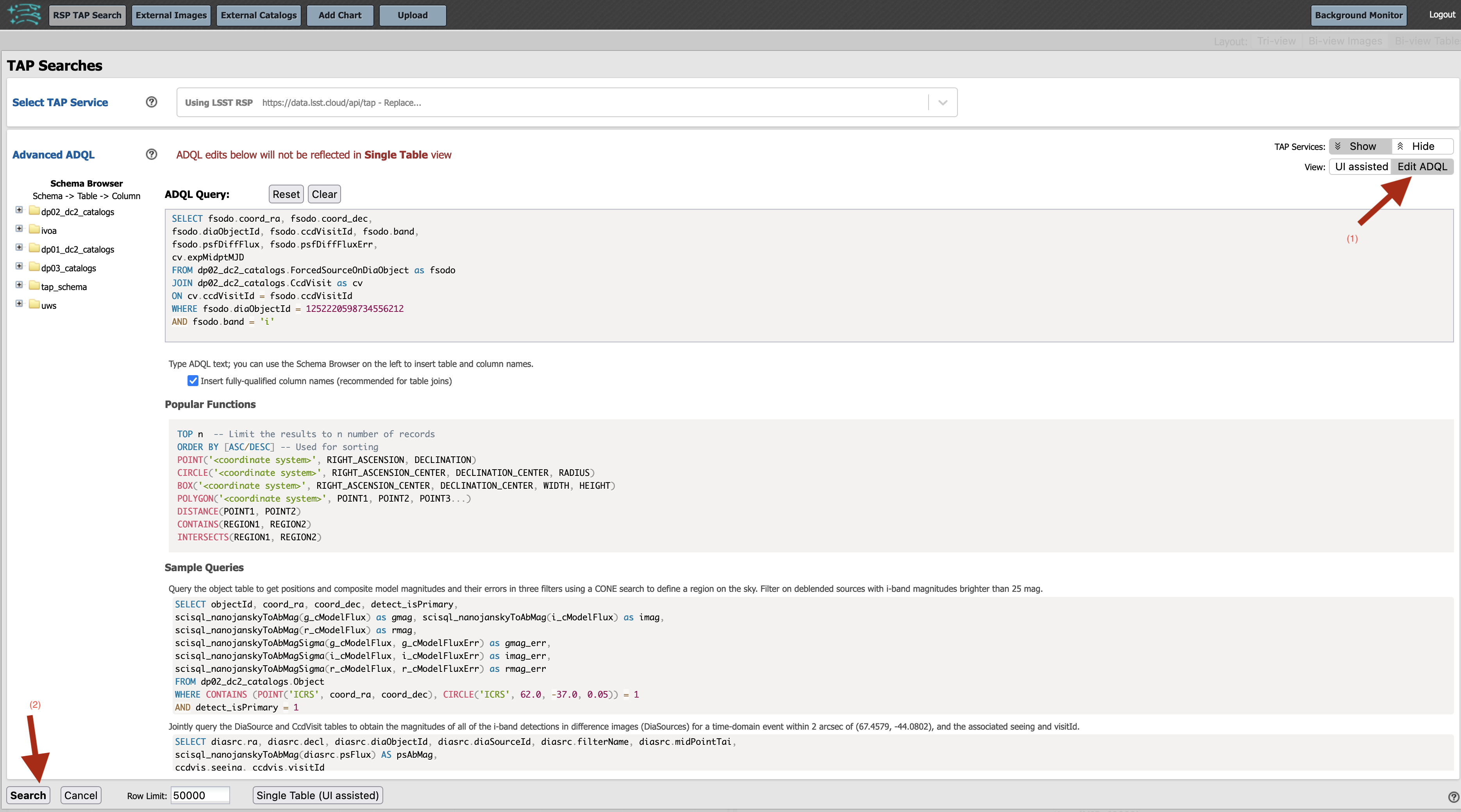
Figure 1: RSP Portal aspect with “DP0.2 catalogs” selected.
1.3. In the ADQL Query box, enter the query as below.
This query will retrieve the coordinates, DIA object identifier, CCD visit identifier, band, and forced difference-image flux
and its error for all rows of the ForcedSourceOnDiaObjects table which are associated with the diaObject of interest,
for i-band visits only.
It also retrieves the exposure time midpoint modified julian date for all visits by joining to the CcdVisit table.
SELECT fsodo.coord_ra, fsodo.coord_dec,
fsodo.diaObjectId, fsodo.ccdVisitId, fsodo.band,
fsodo.psfDiffFlux, fsodo.psfDiffFluxErr,
cv.expMidptMJD
FROM dp02_dc2_catalogs.ForcedSourceOnDiaObject as fsodo
JOIN dp02_dc2_catalogs.CcdVisit as cv
ON cv.ccdVisitId = fsodo.ccdVisitId
WHERE fsodo.diaObjectId = 1252220598734556212
AND fsodo.band = 'i'
Note: The ForcedSourceOnDiaObject table contains forced photometry on both the difference image,
psfDiffFlux, and the processed visit image (PVI; “direct” image), psfFlux.
As this tutorial is using a supernova it uses the psfDiffFlux, which is the forced photometry on the difference image,
in which the static-sky component (the host galaxy) has been subtracted.
However, the psfFlux would be more appropriate for generating the lightcurve of a variable star, as there is no
need to subtract the static component (in this case, the variable star’s average flux).
WARNING: Do not use the ADQL function scisql_nanojanskyToAbMag() to convert difference image fluxes to magnitudes.
This is very dangerous!
This function does not return any value for a negative flux, and difference image fluxes can be negative (e.g., either the
object has declined in brightness compared to the template, or it is a non-detection and the flux is very small and negative).
Using the scisql_nanojanskyToAbMag() function on columns like psfDiffFlux can result in missing data.
While it is generally safe to convert forced fluxes from the PVI to magnitudes, there might be edge cases where the direct image
forced photometry is negative
(e.g., rare cases where the source is faint or gone and in a region of slightly oversubtracted sky background).
It is only ever fully safe to use this function when using SNR > 5 detections in PVIs.
1.4. Click “Search”.
1.5. Set the view of the “Results” panel by clicking on the “hamburger” icon (three horizontal lines on the top left). Click on the double-arrow in the “Results Layout” box, and click on the “Coverage Charts Tables” box. In the results view, see that the query has returned forced flux measurements in the table (right hand side of the figure below), and the “coverage” panel on the left-hand side.
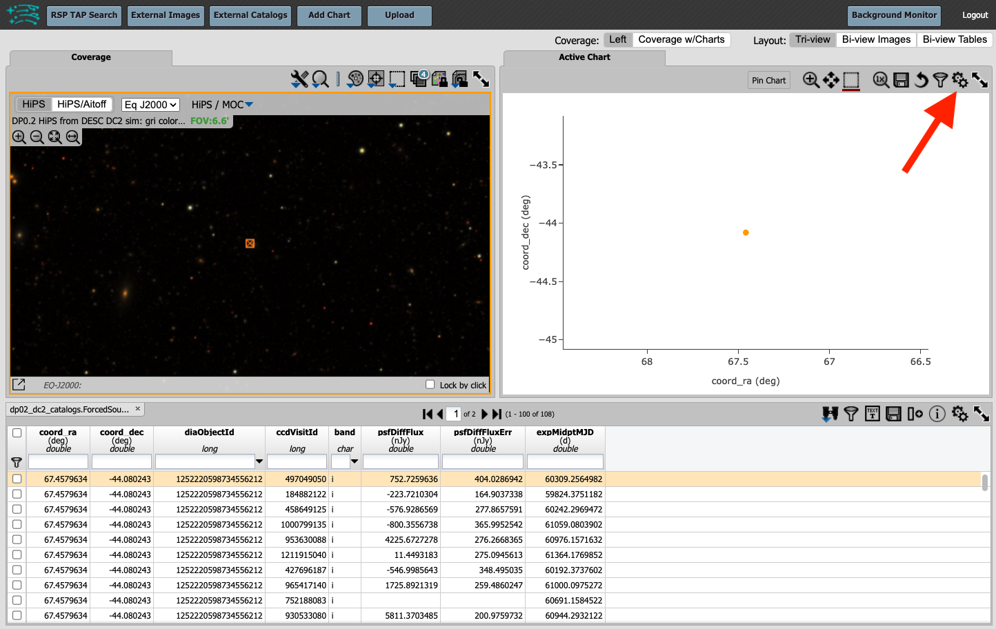
Figure 2: Screenshot illustrating the results of the query, with the selection of “coverage” on the left, and “table” on the right.
1.6. To plot the lightcurve instead of the “coverage” image (default), click on the “Active Chart” tab. The defalt plot will be the dec vs. RA (the plotting chart defaults to plot the data in the two leftmost columns of the table). To change the plot, open the plot parameters pop-up window by clicking on the settings icon (a single gear above the plot window).
1.7. Update the plot parameters as shown in the figure below. Note that the grid line in the y-axis is selected. Click “Apply”. Note how the grid lines in the y-axis illustrate that “off-peak” (non-detection) forced fluxes can be negative.

Figure 3: Plot parameters selection in the pop-up window, set to display the i-band lightcurve.
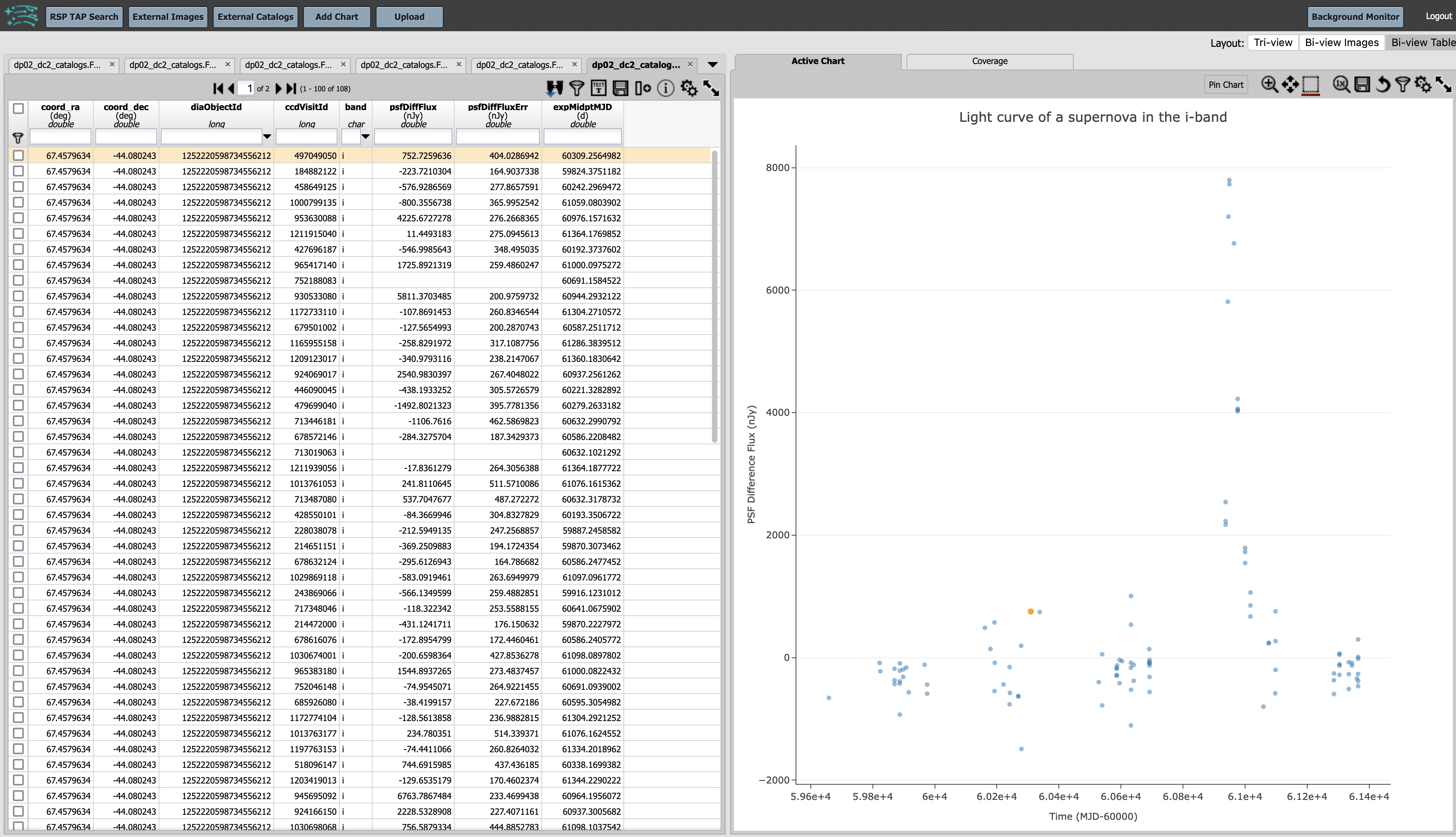
Figure 4: Results view showing the table and the i-band light curve.
1.8. Restrict the x-axis (MJD range) to only show the lightcurve around the dates of peak brightness:
reopen the plot parameters pop-up window, and under Chart Options set the X Min to be 930 and X Max to be 1010.
The result can be directly compared to the lightcurve in Portal Tutorial 2.
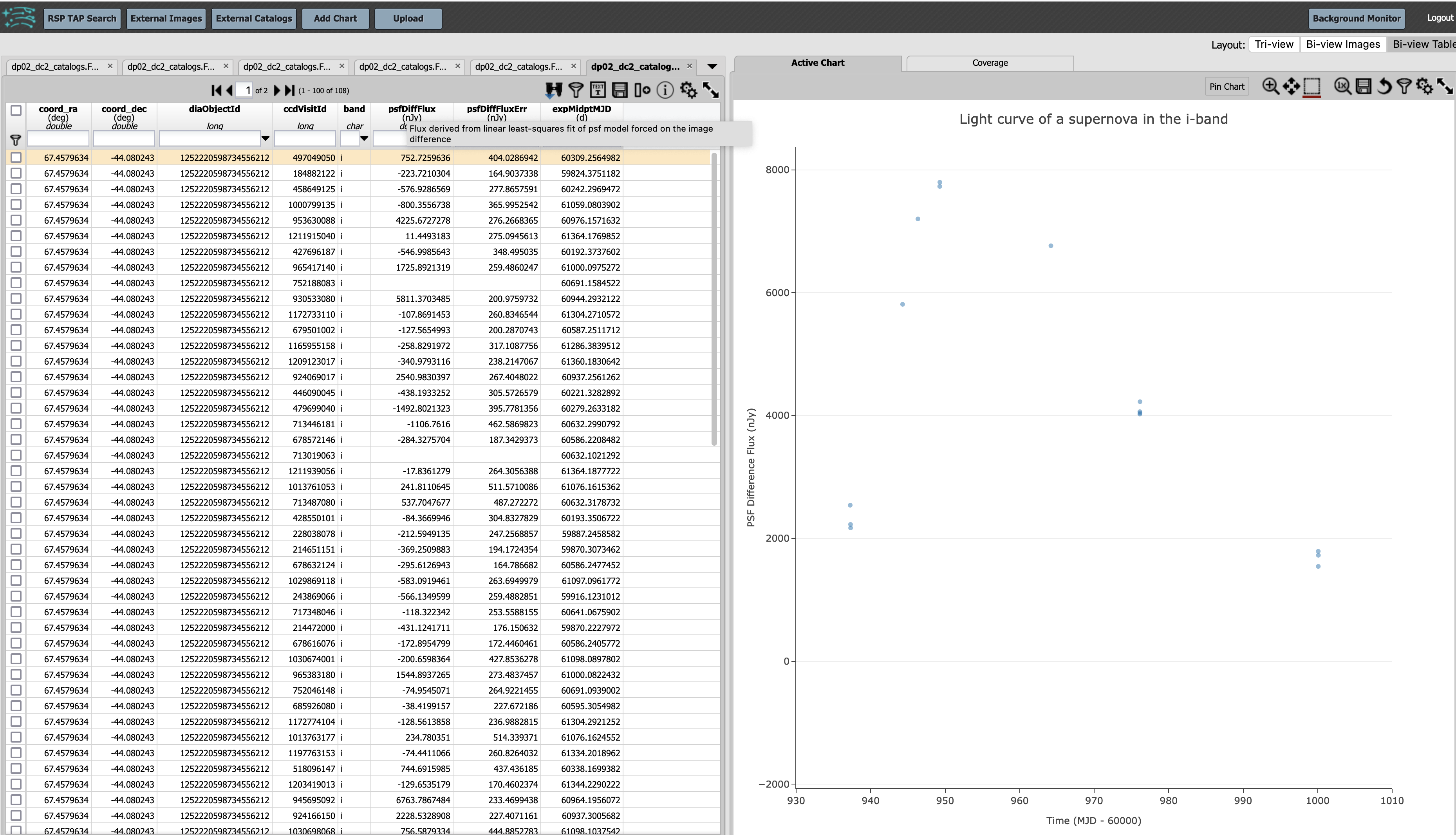
Figure 5: Light curve of the supernova over the limited date range, around the time of the presumed explosion.
Note: A statistical analysis of the lightcurve (e.g., goodness-of-fit to a template; timeseries features) is currently not possible in the Portal, and should be done in the Notebook Aspect.
Step 2. Plot a multi-band lightcurve
NOTE: The Portal does not yet have the built-in functionality to plot a multi-band lightcurve (i.e., to color lightcurve points by their bandpass and add a legend). What follows is a demonstration of a temporary work-around for Portal users: convert the band (u, g, r, i, z, or y) into an ASCII value (e.g., 121, 114, 105) and then set a colorbar for the points based on these values. For the Notebook Aspect, see tutorial notebook 07a and 07b for multi-band lightcurve demonstrations.
2.1. Return to (or start at, if Step 1 was skipped) the ADQL Query interface and enter the query below.
Note that the only difference here compared to Step 1 is that the last line (AND fsodo.band = 'i') is missing,
so that data for all bands will be returned.
SELECT fsodo.coord_ra, fsodo.coord_dec,
fsodo.diaObjectId, fsodo.ccdVisitId, fsodo.band,
fsodo.psfDiffFlux, fsodo.psfDiffFluxErr,
cv.expMidptMJD
FROM dp02_dc2_catalogs.ForcedSourceOnDiaObject as fsodo
JOIN dp02_dc2_catalogs.CcdVisit as cv
ON cv.ccdVisitId = fsodo.ccdVisitId
WHERE fsodo.diaObjectId = 1252220598734556212
2.2. Follow steps 1.4, 1.5, and 1.6 to plot the multi-band lightcurve with identical color markers for all bands. The plot will appear as in the left hand side of the figure below. Note that there are many more points on the new plot, because all bands are included instead of just i-band.
2.3. The work-around to plot the measurements in various bands in different colors is to convert the band (u, g, r, i, z, or y) into an ASCII value (e.g., 121, 114, 105).
This starts with adding a column, and setting it to be the ASCII value of the band column.
To add a new column, click the 5th icon in the results table (the vertical rectangle with a + sign), as shown in the figure below.
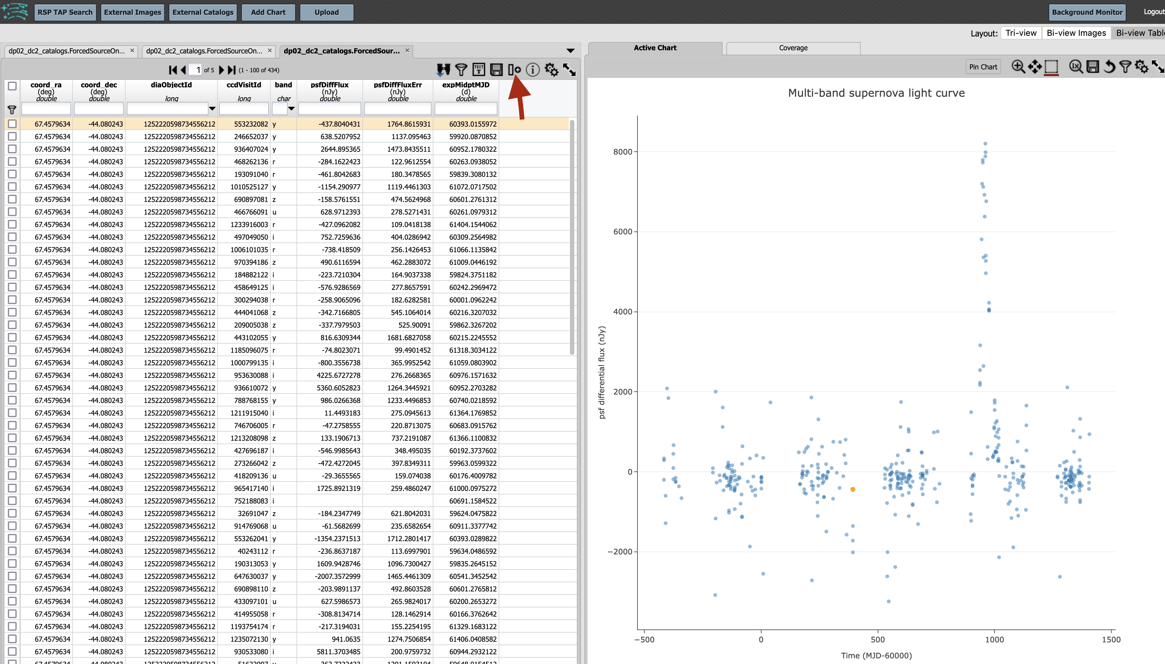
Figure 6: Multi-band light curve of a supernova with symbols for all bands plotted in the same color.
2.4. In the “Add a column” pop-up window, enter a name for the new column (bands_ascii) and the expression to convert
the character in column band into its ASCII value: ascii("band").
Set the “Data Type” to long, then click on “Add column”, as shown in the figure below.
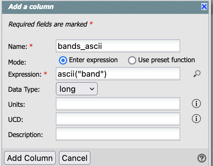
Figure 7: Parameters for the new column, needed to plot different filter bands in different colors.
2.5. In the results view, see the new column in a numeric format: the corresponding ASCII value of the character in the band column.
In the figure below, the new column named bands_ascii is marked with a red arrow.
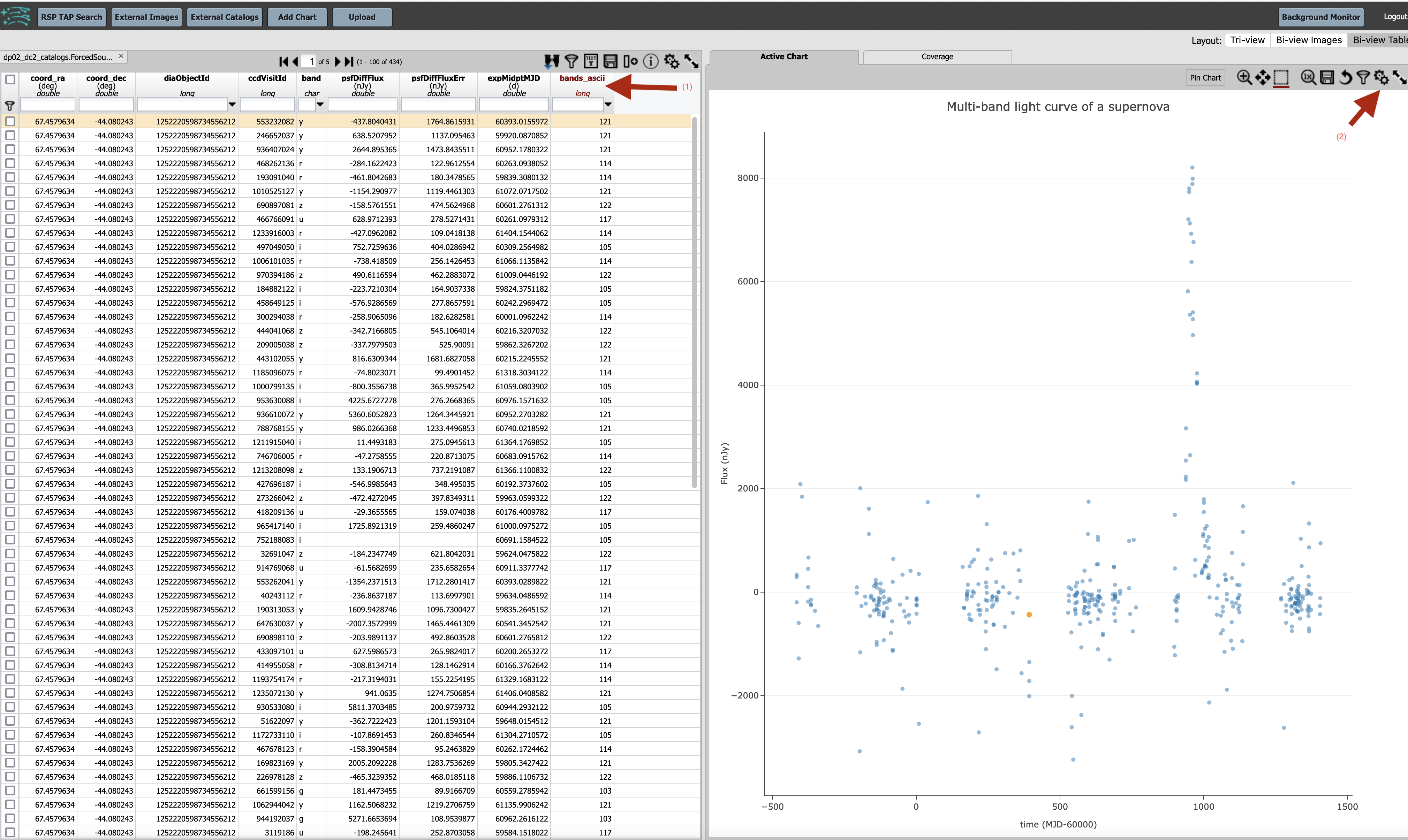
Figure 8: New column in the table, resulting from the step above.
2.6. Set the colorbar for the points based on the values in the new column bands_ascii.
Open the “Plot Parameters” pop-up window by clicking on the settings icon (single gear in the plot panel).
Under “Trace Options” enter “bands_ascii” for the “Color Map” and “Rainbow” for the “Color Scale”, as shown in the figure below.
Click “Apply”.
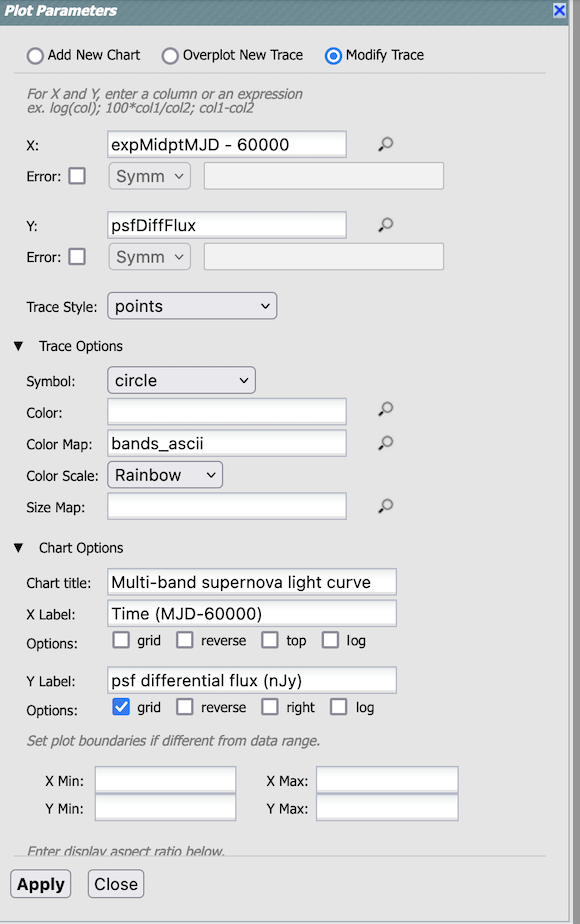
Figure 9: Plot parameters to enable the view multi-band supernova light curve in distinct colors.
2.7. View the new version of the lightcurve with the points colored by band, as in the figure below.
Use the mouse to hover-over points in the plot, and notice that the pop-up info box for a given point includes only the
data included in the plot: x-axis value, y-axis value, and the bands_ascii value.
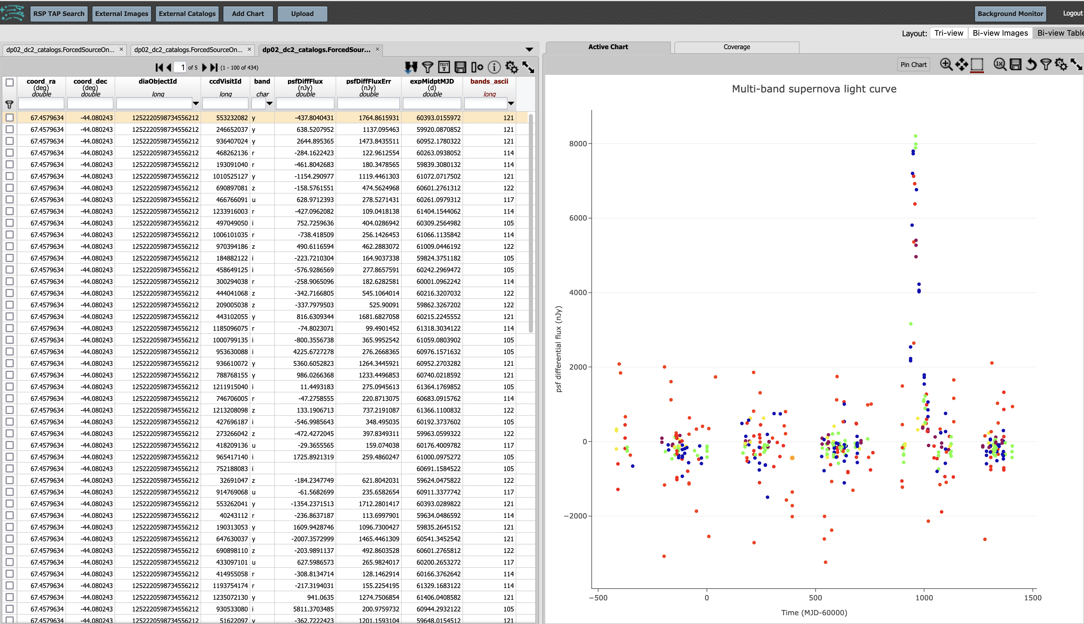
Figure 10: Multi-band lightcurve of the supernova with points colored by band.
2.8. Restrict the multi-band lightcurve back down to a single filter without redoing the ADQL query.
Apply a single r filter by clicking on the drop-down arrow in the band column header, adding a check-mark by the r entry, and clicking on “Apply.”
Do it again for g, and notice that additional points appear, in different colors.
You can check or uncheck as many filters as you wish.
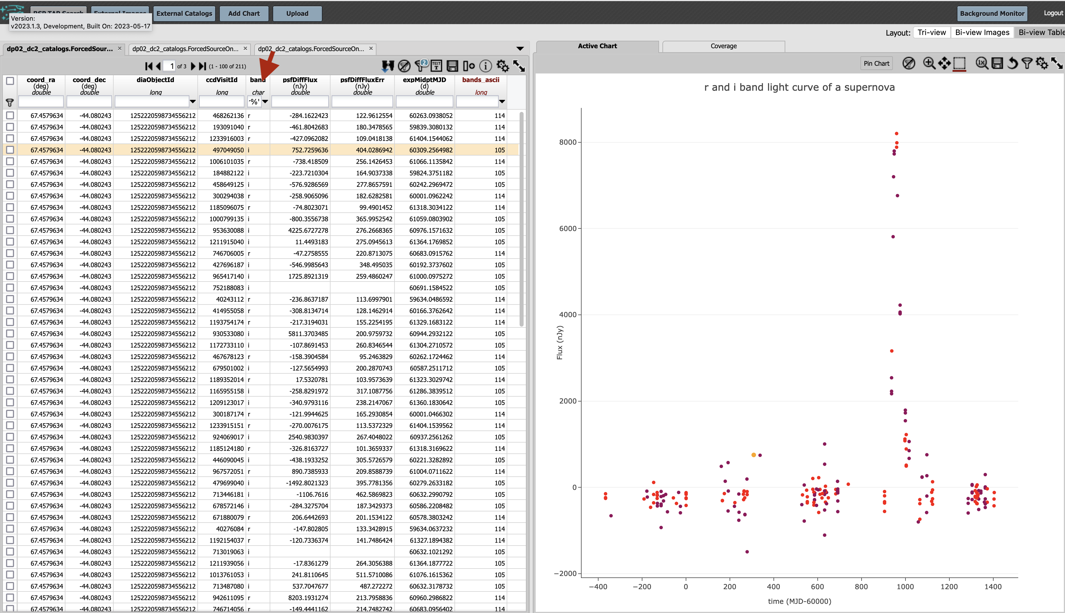
Figure 11: Supernova light curve in two filters, as selected in the drop-down menu.
Note: While not being able to choose your own symbols or colors for data points on the plot is a temporary drawback of the Portal, the future releases will bring improved functionality.
Step 3. Exercises for the learner
3.1. Add error bars to the lightcurve.
3.2. Try another supernova and follow the steps above (e.g., use diaObjectId = 1250953961339360185).