04. Exploring Extended Object Populations with Histograms

RSP Aspect: Portal

Contact authors: Melissa Graham and Greg Madejski

Last verified to run: 2025-01-09

Targeted learning level: intermediate

Introduction: This tutorial demonstrates how to retrieve apparent magnitudes and cluster offsets for a sample of extended objects around a rich galaxy cluster. It also demonstrates how to create 1-dimensional (1D) and 2-dimensional (2D) histograms to explore their apparent magnitude and color distributions. Galaxy color-magnitude diagrams (CMDs) are a standard and widely-used diagnostic plot type in astronomy. This tutorial uses a galaxy CMD that plots the g-band magnitude on the X-axis and the g-r color on the Y-axis.

This tutorial assumes the successful completion of the beginner-level Portal tutorial 01, and uses the Astronomy Data Query Language (ADQL), which is similar to SQL (Structured Query Language). Learners who are unfamiliar with galaxy CMDs might find Wikipedia’s galaxy color-magnitude diagram page a helpful introduction to their red sequence, blue cloud, and green valley components.

This tutorial uses cModel fluxes (Composite Model).

For more information about the DP0.2 catalogs, tables, and columns, visit the DP0.2 Data Products Definition Document (DPDD) DP0.2 Data Products Definition Document (DPDD) or the DP0.2 Catalog Schema Browser.

Step 1. Execute the ADQL query

1.1. Log in. Log into the Portal Aspect then click on the “DP0.2 Catalogs” Tab in the top menu.

1.2. Select “Edit ADQL”. At upper right, click “Edit ADQL” to toggle from the default “UI assisted” interface to the ADQL interface.

1.3. Enter the ADQL statement. Copy-paste the following ADQL code into the “ADQL Query” box.

SELECT coord_dec, coord_ra, detect_isPrimary,
scisql_nanojanskyToAbMag(g_cModelFlux) as gmag,
scisql_nanojanskyToAbMag(r_cModelFlux) as rmag,
g_extendedness as gext,
r_extendedness as rext,
DISTANCE(POINT('ICRS', coord_ra, coord_dec), POINT('ICRS', 55.75, -32.27)) as radial_offset
FROM dp02_dc2_catalogs.Object
WHERE CONTAINS(POINT('ICRS', coord_ra, coord_dec), CIRCLE('ICRS', 55.75, -32.27, 1.0)) = 1
AND detect_isPrimary = 1
AND g_extendedness = 1
AND r_extendedness = 1
AND scisql_nanojanskyToAbMag(g_cModelFlux) < 25
AND scisql_nanojanskyToAbMag(r_cModelFlux) < 25

1.4. Understand the columns selected. The ADQL statement above will retrieve the RA and Dec coordinates (coord_ra, coord_dec), the detect_isPrimary flag, the apparent g- and r-band magnitudes (converted from the measured cModel fluxes), the extendedness flag in the g- and r-bands (g_extendedness and r_extendedness), and each objects’ two-dimensional sky distance from the search coordinates (radial_offset).

1.5. Understand the query constraints. The ADQL statement above applies a spatial constraint that only objects within 1 degree of the center of a known cluster at RA = 55.75 deg and Dec = -32.27 deg are returned. Returned objects must also have a detect_isPrimary flag equal to 1 (for deblended, non-duplicated objects only), extendedness flags equal to 1 in the g- and r-band filters (for extended, not point-like objects only), and g- and r-band apparent magnitudes brighter than 25. Together these conditions will return only bright, deblended, extended objects (i.e., individual galaxies).

1.6. Increase the row limit and execute the query. At bottom left, increase the “Row Limit” to 300,000, and click “Search”.

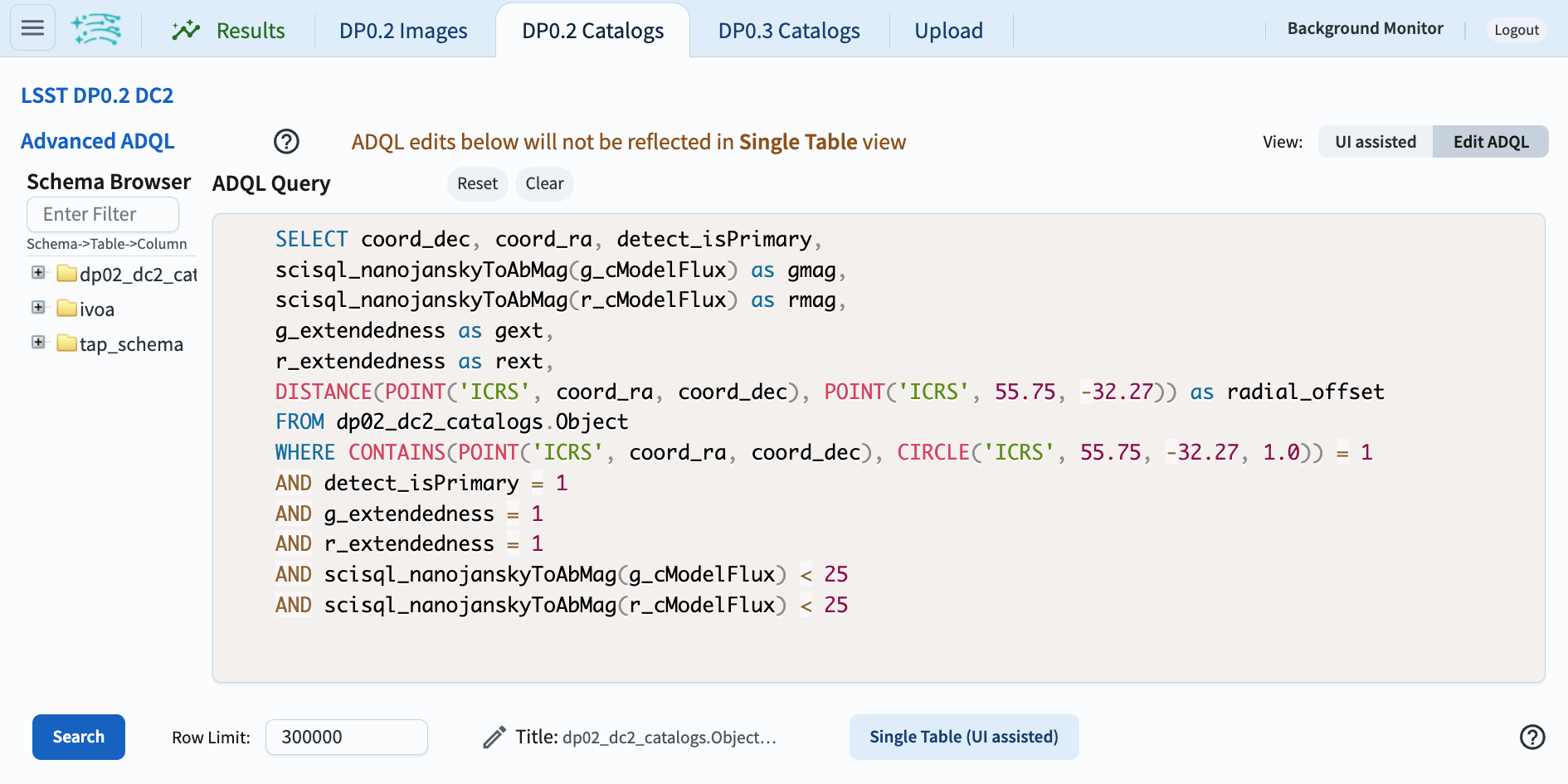
Figure 1: The Portal’s ADQL interface with the query entered and the row limit updated to 300,000.

1.7. The query will return 227,752 objects.

Step 2. Explore the default results layout

2.1. Three-panel results view. The default layout for the Results tab is shown in Figure 2, below. If any of the panels are missing, switch to the default layout by clicking the menu icon at upper left (three horizontal bars), then click the layout icon under “Results Layout”, and choose the triple view that matches Figure 2.

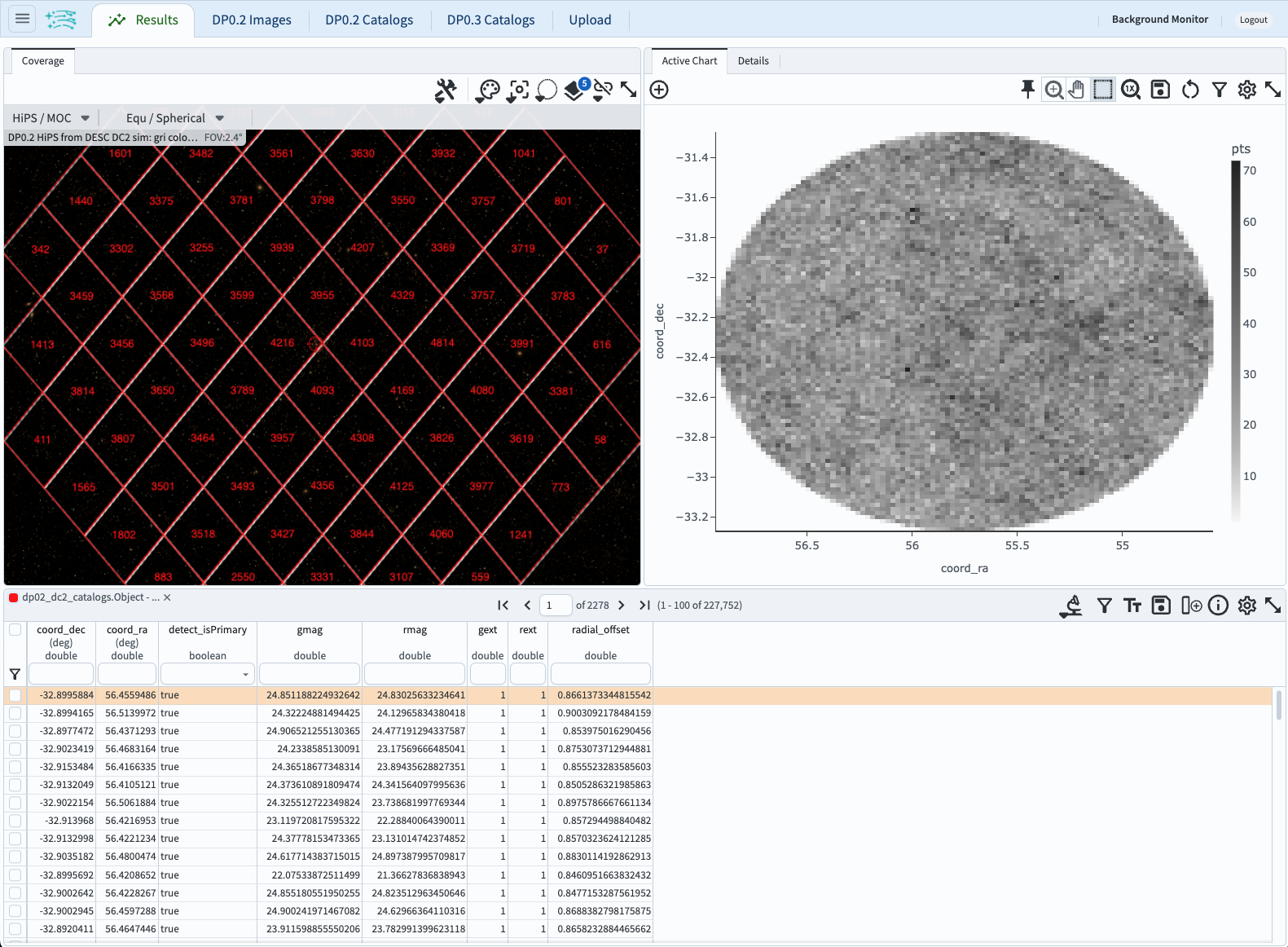
Figure 2: The three-panel default results layout of coverage chart (upper left), active chart (upper right), and table (below).

2.2. Zoom in on the coverage chart. At upper left, in the coverage chart window, a HEALpix grid maps the number of returned objects per region. Zoom in by clicking on the magnifying glass icon with the + sign until individual markers appear.

2.3. Filter on radial offset. In the table header row with the funnel icon at left, apply a filter that constrains the radial_offset to be less than 0.03 degrees (type “< 0.03” into the box and press “enter” or “return” on the keyboard). Note that, in the coverage chart, only galaxies that look like cluster members now have markers, as shown in Figure 3.

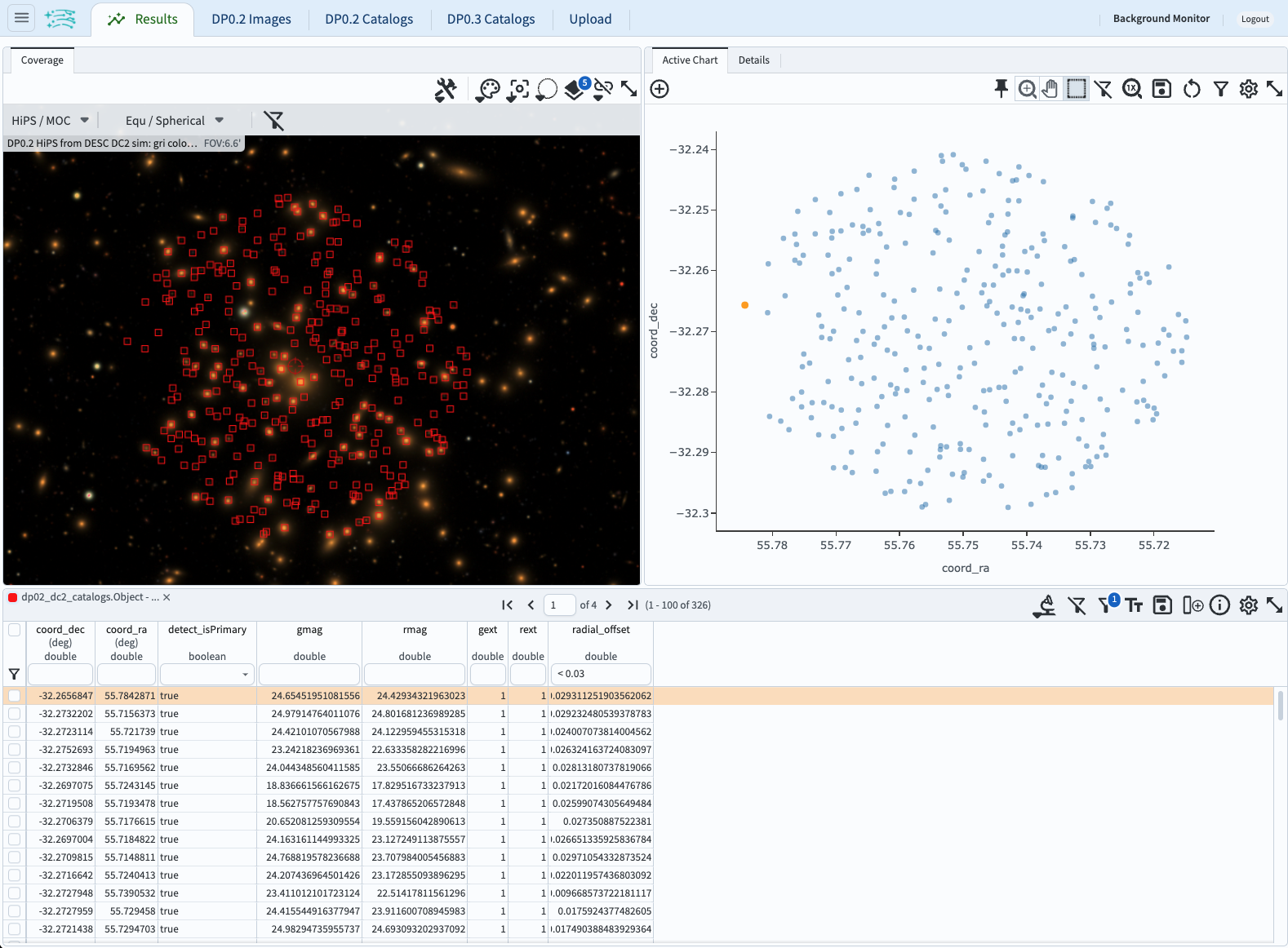
Figure 3: After applying a filter on the radial offset column, all three panels automatically update.

2.4. Remove the filter. Delete the constraint “< 0.03” on radial_offset and press “enter” or “return” on the keyboard to remove the filter.

Step 3. Create a CMD as a 2D histogram

3.1. Add a CMD as a new trace. At upper right, in the active chart panel, click the gear icon to open the “Plot Parameters” pop-up window. Select “Overplot New Trace”, which means to plot another set of values on the current plot. Fill in the boxes as shown in Figure 4 to plot the g-r color magnitude diagram (CMD). Note that “heatmap” is a term for 2D histogram.

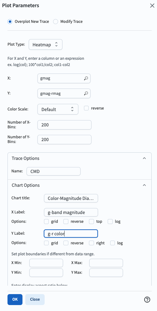
Figure 4: The plot parameters pop-up window showing how to add a new trace, which plots galaxy color versus magnitude.

3.2. View the active chart panel. The plot now has two heatmaps (two 2D histograms): the original of Decl versus RA in greyscale, and the newly added CMD in blue/red. This is not very useful! The purpose of showing this weird plot is to demonstrate the flexibility of the Portal’s plotting capabilities.

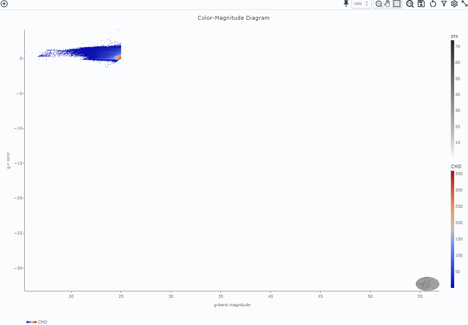
Figure 5: The active chart panel with two 2D histograms co-plotted: the original coordinates heatmap in grey and the color-magnitude heatmap in blue/red.

3.3. Remove the default trace (coordinates). Click on the gear icon to open the plot parameters pop-up window. Choose “trace 0” and click “Remove Active Trace”. In the next pop-up window click “OK”, as shown in Figure 6.

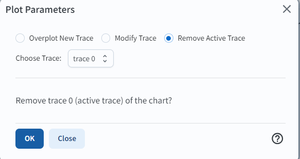
Figure 6: The pop-up window to remove the selected trace.

3.4. View the CMD. The active chart panel should now appear as in Figure 7. Note the sharp cutoffs at the bright end (around g=17, g-r=0.5) and the faint end (around g=24.5, g-r=0.2), due to the constraints applied in the ADQL query. Recall also that DP0.2 data set is based on a simulation, and that a real LSST color-magnitude diagram for galaxies might look quite different.

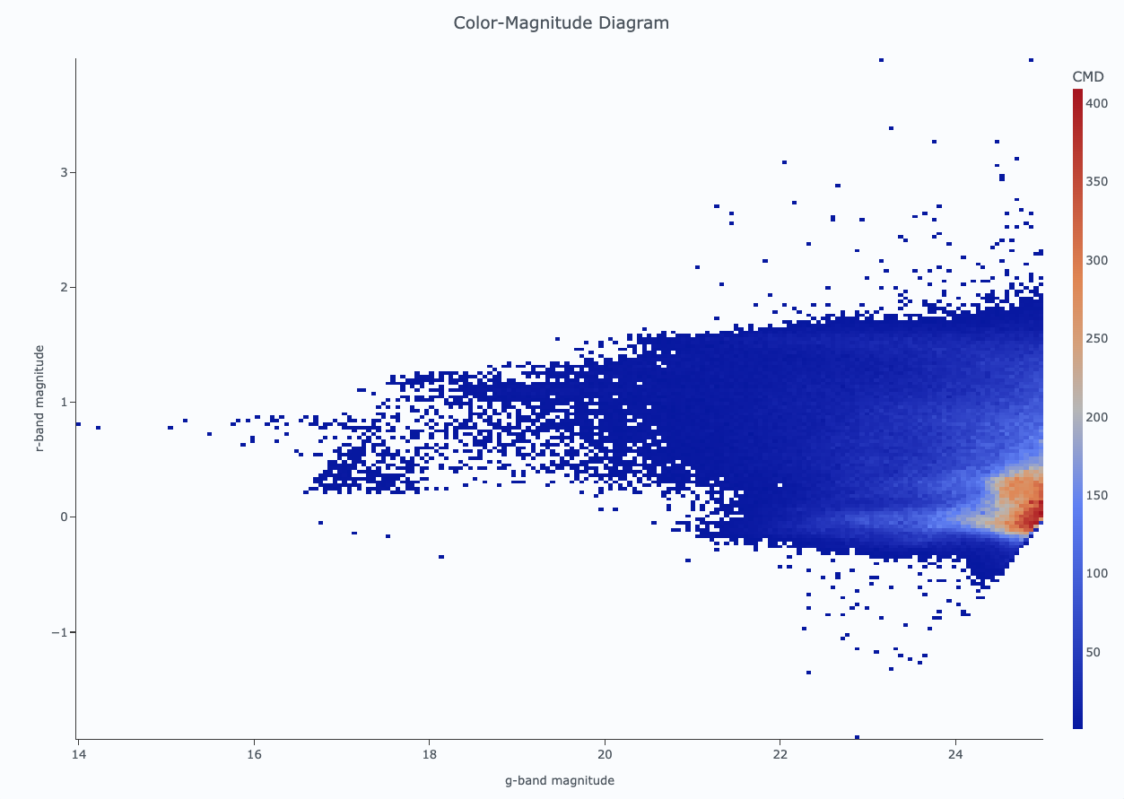
Figure 7: The color magnitude diagram (CMD) as a 2D histogram (heatmap) for all returned objects.

Step 4. Add magnitude distributions as 1D histograms

4.1. Add a new chart. In the upper left corner of the active chart panel, click on the plus sign in a circle to add a new chart. Select type “Histogram” from the drop-down menu, and set the other boxes to match Figure 8. To open the color picker and choose a green color for the g-band, click on the magnifying glass in the “Color” field. Click “OK” in the color picker, then “OK” in the “Add a new chart” window.

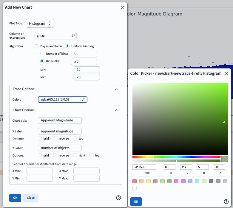
Figure 8: The parameters to use to create a new chart (new plot) containing the g-band apparent magnitude distribution.

4.2. Notice the histogram options available. As shown in Figure 8, this tutorial uses “uniform binning” (the same size for all bins), but “Bayesian blocks” is also an option (quantiles defined by the data itself). This tutorial sets the bin sizes, and first and last bin edges, but there is also the option to simply set the number of bins and those values will be worked out automatically.

4.3. View the g-band magnitude distribution. It should appear as in Figure 9.

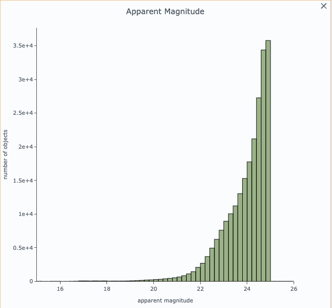
Figure 9: The g-band apparent magnitude distribution as a 1D histogram.

4.4. Add the r-band apparent magnitude distribution to the new plot. With the 1D histogram plot selected, click on the single gear icon at upper right. (The selected plot will have an orange outline; click on the plot to select the plot.) In the “Plot Parameters” pop-up window, select “Overplot New Trace”, and fill in the boxes as in Figure 8 except use the rmag instead of gmag column and choose an orange color. Click “OK” to add the trace of the r-band apparent magnitude distribution to the plot.

4.5. Review the 1D histograms. The apparent magnitude distributions should appear as in Figure 10.

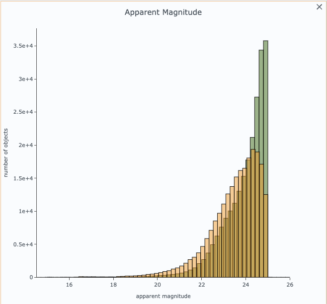
Figure 10: The final 1D histograms of the apparent magnitude distributions.

4.7. Known issues: the fact that the legend is not automatically appearing once there are multiple traces in a single plot is a known issue.

Step 5. Restrict all plots to objects near the rich cluster

5.1. Filter on radial offset. Similar to step 2.3, but use a slightly larger maximum radius of 0.05 degrees: enter “< 0.05” into the filter entry box in the table for the radial_offset column and press “enter” or “return” on the keyboard.

5.2. Notice the 2D CMD cannot be displayed. There are now too few objects (790 objects) to populate a 2D histogram.

5.3. Create a new chart with a scatter-plot CMD. In the upper left corner of the active chart panel, click on the plus sign in a circle to add a new chart. Fill in the options as shown in Figure 11 and click “OK”.

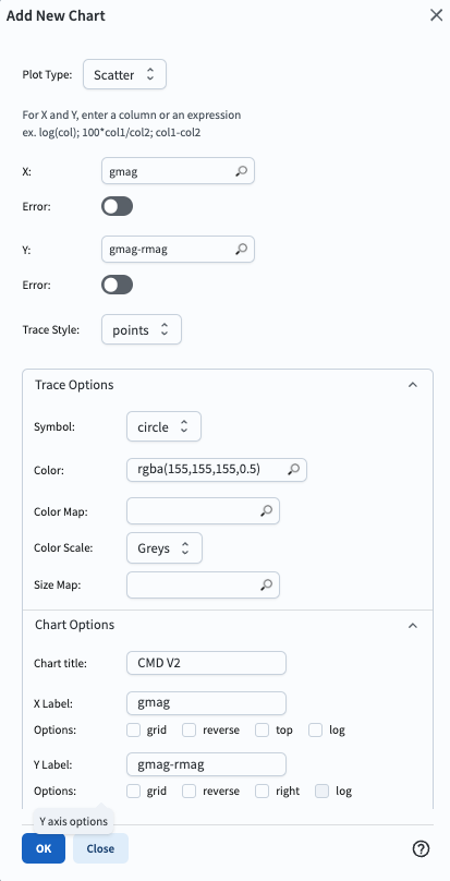
Figure 11: The parameters to use to create a new chart (new plot) containing the galaxy CMD as a scatter plot. For color, select the light grey palette box.

5.4. Find the cluster red sequence. In the new galaxy CMD scatter plot at right in Figure 12, the cluster red sequence can be seen as an overdense locus of points.

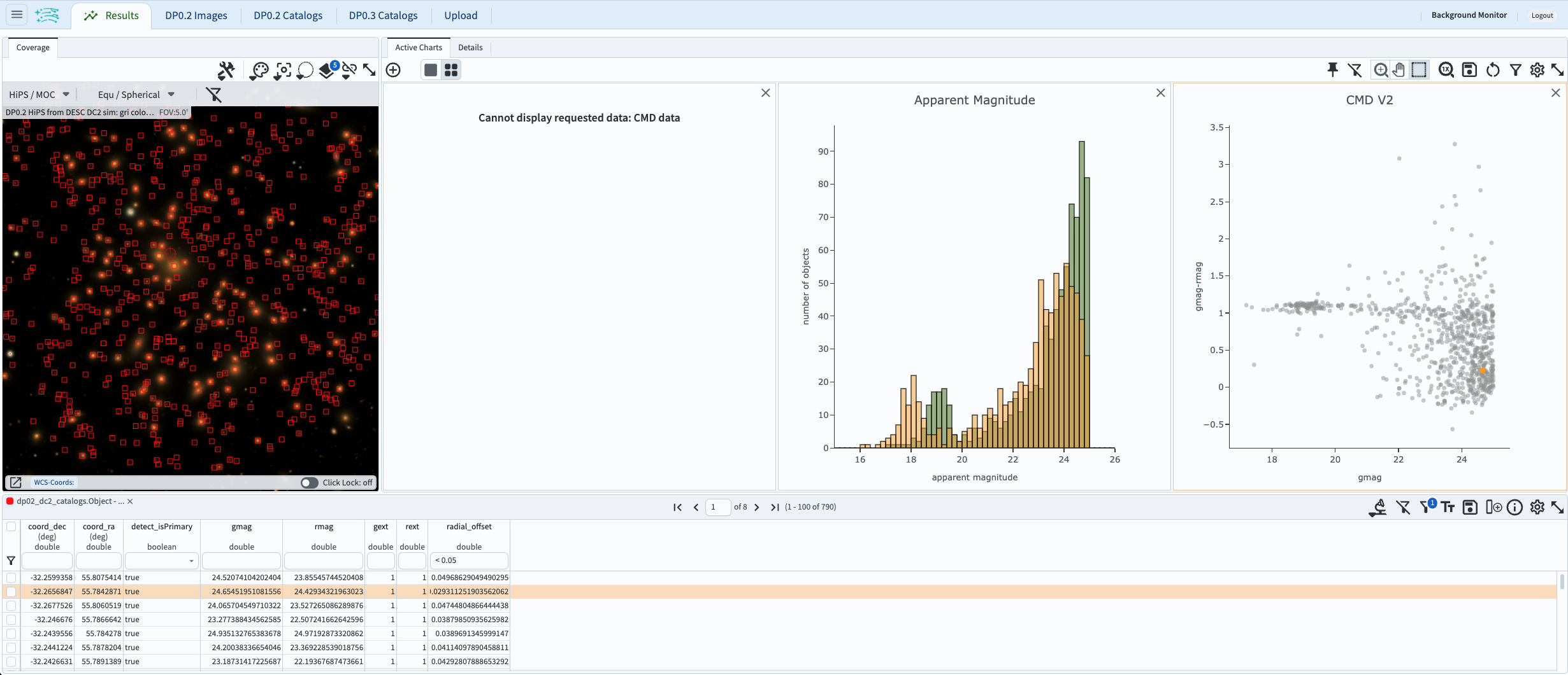
Figure 12: The full Results view tab with three plots in the active chart, the right-most one being a scatter plot CMD for galaxies near the center of a known rich cluster, and the cluster’s “red squence” highlighted with a box (added after the screenshot was acquired).

5.5. Remove the filter. Delete the constraint “< 0.05” on radial_offset and press “enter” or “return” on the keyboard to remove the filter. All three plots in the active chart will refresh to include all objects.

Step 6. Exercises for the learner

6.1. Return to the ADQL query in step 1.3, and re-do this tutorial but include faint extended objects down to 28th magnitude. Notice how the histograms change in shape.

6.2. Return to the ADQL query in step 1.3, and add u, i, z, and y-bands to the retrieved columns. Create an apparent magnitude histogram with all six filters. Create a color-magnitude diagram (or a color-color diagram) with the bands of your choice.