03. View a SNIa Host Galaxy (intermediate)
RSP Aspect: Portal
Contact authors: Melissa Graham
Last verified to run: 2024-05-01
Targeted learning level: intermediate
Introduction: This portal tutorial demonstrates how to get an initial look at the potential host galaxy of a SNIa in the six (ugrizy) deepCoadd images.
This tutorial assumes a basic working knowledge of the Portal interface (e.g., review of the Image Search (ObsTAP) instructions or the successful completion of the first Portal tutorial). For more information about the DP0.2 catalogs and images, visit the DP0.2 Data Products Definition Document (DPDD).
1. Query for Images
1.1. Log into the Portal Aspect, click on “DP02 Images” tab at the top.
1.2. Under “Observation Type and Source”, choose “Calibration Level” 3, which is for derived images such as deepCoadds and difference images. Leave the other options to their default settings except for the “Data Product Subtype” enter “lsst.deepCoadd_calexp”.
1.3. Under “Location”, choose “Observation boundary contains point” from the drop-down menu and enter the coordinates “67.4579, -44.0802” - the known location of the SNIa from Portal tutorial 02.
1.4. Do not set any timing or spectral coverage constraints, and do not change the default table column selections.
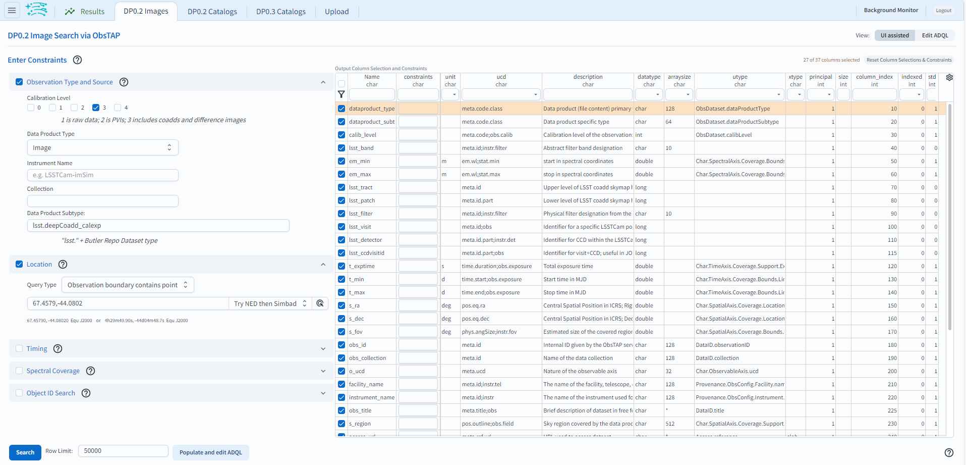
Query for the deepCoadds that cover the SNIa location.
1.5. Click “Search”.
2. Interact with the deepCoadds
2.1. On the right hand panel, click on “Data Product: ivoa…” tab, then click on the grid icon (hover-over text “Tile all images in the search result table”) to simultaneously view all six filters’ deepCoadds. The default view is to center all deepCoadds on the center of the patch. In this example the compass (Under Layers, click “Show the directions of Equatorial J2000 North and East) has been enabled using the “Tools” icon (wrench and hammer, hover-over text “Tools drop down: save, rotate, extract and more”).
2.2. Click on the hamburger icon at the upper left near the Rubin logo to select “Tables, Coverage Images Charts” in the Results Layout section to show just one image and the table side-by-side. To display the six filters’ deepCoadds, select “Data Product: ivoa.ObsCore…” tab on the right side panel.
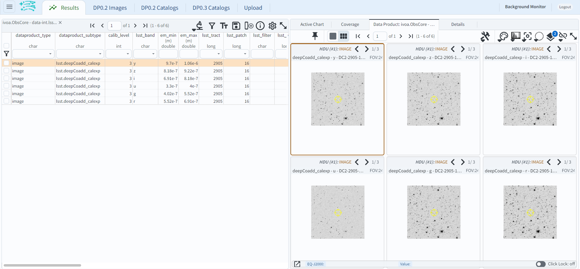
The default view centers the image display on the patch center.
2.3. Align and lock by WCS. Click on the down arrow on the “align” icon (chain with a slash) above the six images on the right panel, (hover-over text “Image alignment drop down…”) and under “Align and Lock Options” select “by WCS”. Notice now that zooming and panning in one image does the same in all six images.
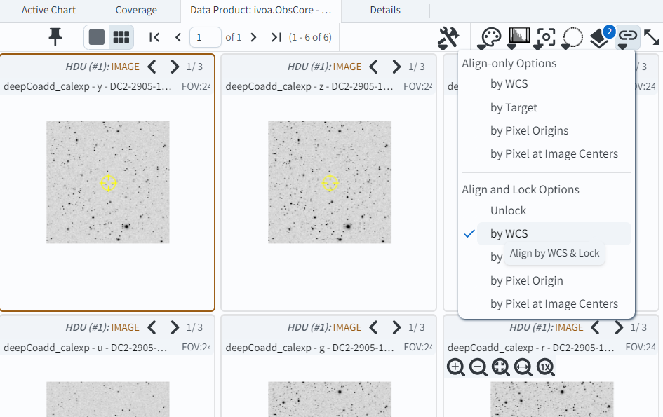
Choose to align and lock on WCS.
2.4. Mark and center the SNIa. Choose the “center” icon (hover-over text “Image center drop down”), and in the box next to “Center On” enter the SNIa’s coordinates, “67.4579, -44.0802”, and then click “Go & Mark”. Click the magnifying glass with the “+” symbol to zoom-in on the centered location, and grab and drag to pan around the image. If you happen to pan away from the SNIa, recenter using the “center” icon and finding the SNIa coordinates under “Recent Positions”.
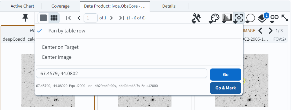
Center on and mark the coordinates of the SNIa.
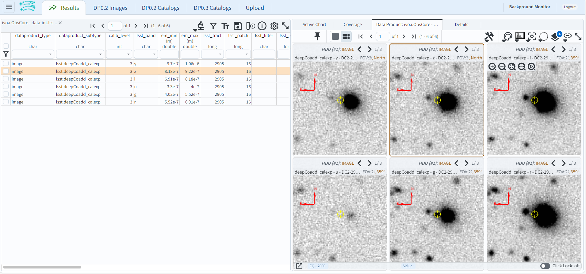
A zoom-in on the SNIa and its host, with linear zscaling.
Notice: In the figure above, the images in the grid are displayed in the order they appear in the table: top row (left to right) then bottom row (left to right). In the table, notice that the filter order is y, z, i, u, g, r. To sort the table so that the filter order is u, g, r, i, z, y, click on the column heading for the “em_min” column.
2.5. Rescale the flux to explore the underlying distribution of host galaxy light. Use the “scale” icon (panel icon with a histogram, third from left, hover-over text “Stretch drop down: change the background image stretch”) to set the Stretch Type to “Log: Stretch to 99%”. (Note: click on “Z Scale Log Stretch”, then select “Log: Stretch to 99%”, if necessary.) Notice that there appears to be a faint - but spatially distinct - extended object at the location of the SNIa, especially in the g-band image (bottom center), which at first was not obvious due to the wings of the brighter galaxy.
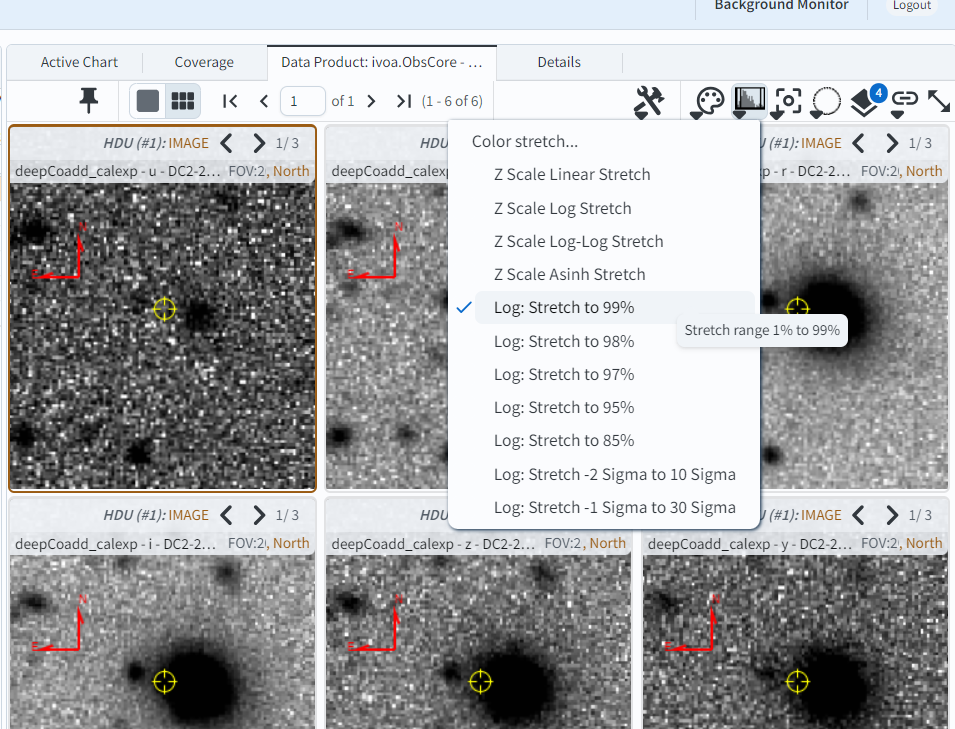
Well the host association looks a little complicated!
Techniques for associating SNIa with their host galaxies are beyond the scope of this tutorial, which was only concerned with getting an initial look at the potential host galaxy.