02. Explore a SNIa Lightcurve (intermediate)
RSP Aspect: Portal
Contact authors: Melissa Graham and Greg Madejski
Last verified to run: 2024-05-14
Targeted learning level: intermediate
Introduction: This tutorial explores the data for a Type Ia supernova (SNIa) lightcurve: the i-band photometry, the seeing for each i-band epoch, and the astrometric scatter of the i-band observations. The scientific motivation here is that a user knows the coordinates of a low-redshift SNIa (67.4579, -44.0802), and now wants to find an i-band epoch in which this SNIa was bright and the seeing was good. The user also wants to get a sense of the scatter in the astrometry for the coordinates in the DiaObject catalog. For example, perhaps the user knows there is pre-explosion JWST imaging of the host galaxy, and is looking for the best image from Rubin Observatory with which to co-register with the JWST image in order to characterize the underlying stellar population at the SNIa’s location. (Note that typically, laser adaptive optics is necessary to obtain ground-based images of SNe that have high enough astrometric precision to co-register with a space-based image and identify a progenitor star, so this use-case is a bit contrived).
This tutorial assumes a basic working knowledge of the Portal interface (e.g., the successful completion of the first Portal tutorial). This tutorial uses the Astronomy Data Query Language (ADQL) to query and retrieve data from the DP0.2 catalogs. ADQL is similar to SQL (Structured Query Language), and the documentation for ADQL includes more information about syntax and keywords. For more information about the DP0.2 catalogs, visit the DP0.2 Data Products Definition Document (DPDD) or the DP0.2 Catalog Schema Browser.
WARNING: In this tutorial, the difference-image fluxes are converted to magnitudes in the TAP query. This is usually safe to do, because supernovae fluxes should never be negative in a difference image – unless the supernova also appears in the template image. In the case of DP0.2, due to how the template images were built, some of the template images are contaminated with supernova flux, potentially up to 40% of DC2 SNIa. This leads to negative-flux difference-image detections that are significant (SNR>5), and thus an overall offset in the SNIa lightcurves. Work is ongoing to evaluate this issue and recommend a robust correction method (see Images). Note that this offset is not discoverable in the following tutorial.
1. Determine the DiaObject Id
1.1. Log in to the Rubin Science Platform, and click on Portal. This will take you to the next screen, where you will have several options. For the purpose of this exploration, you will be using DP0.2 Catalogs, so click on the “DP0.2 Catalogs” tab on top of the screen.
1.2. Click on the box on the screen top where you select the tables - this will show all the available tables. Select dp02_dc2_catalogs.DiaObject table.
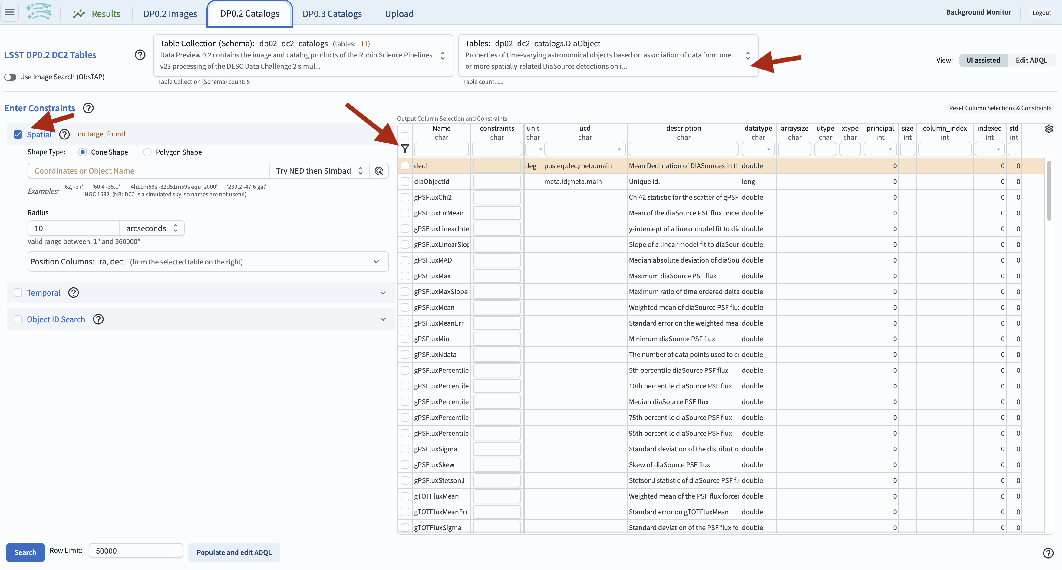
Screenshot of RSP portal start page where the user can select table and constraints.
1.3. On the left-hand side of the screen, under “Enter Constraints” you will have three choices, “Spatial,” “Temporal,” and “Object ID Search.” Select only “Spatial.”
1.4. In the “Spatial” entry, leave the “Shape Type” as the default “Cone shape,” and for “Coordinates or Object Name” enter the coordinates 67.4579, -44.0802. Set the “Radius” to 2 arcsec.
1.5. In the table at right, select columns ra, decl, and diaObjectId to be returned. If you wish to see only the rows selected by you - click on the little funnel.
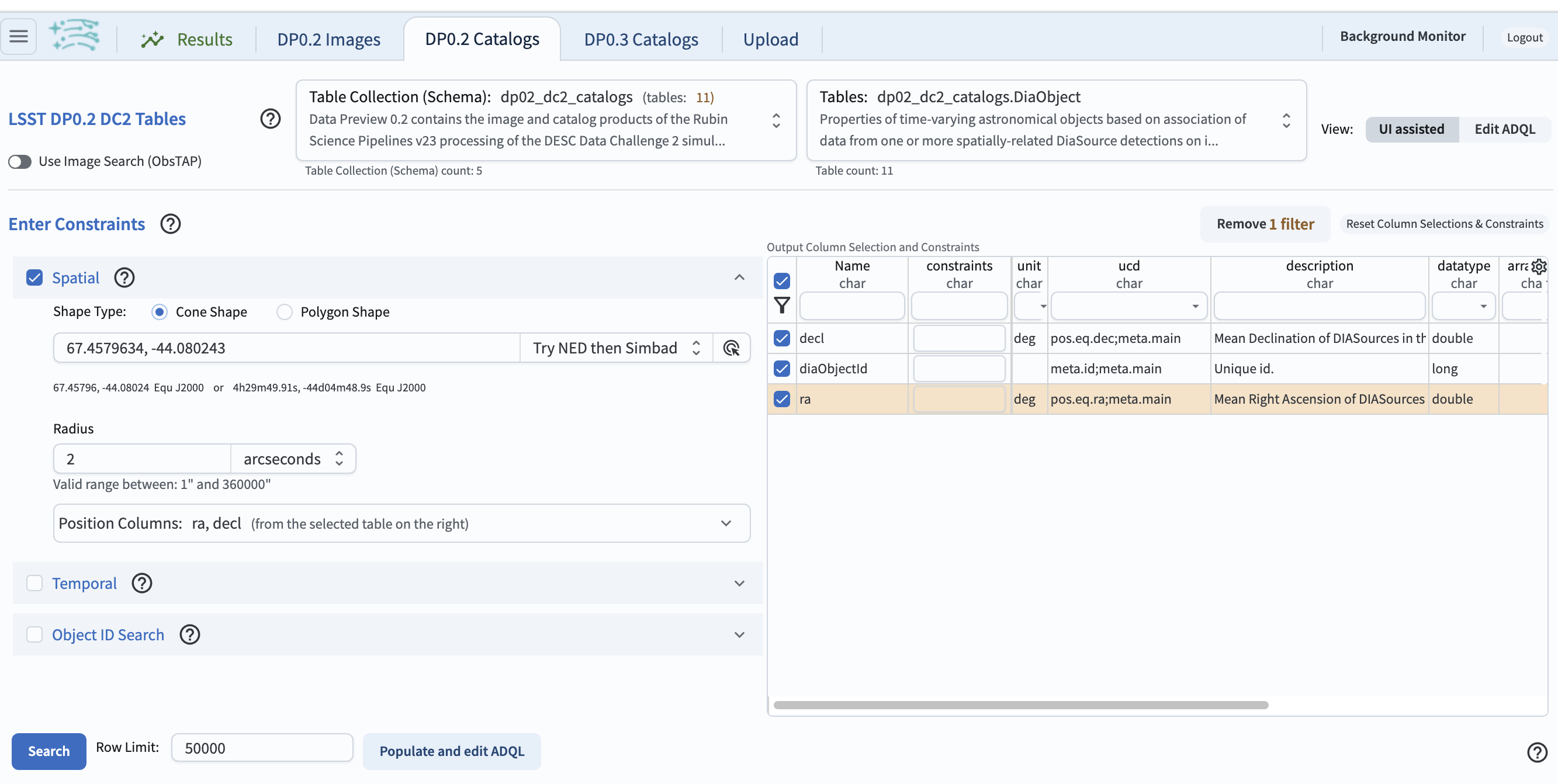
Initial query to obtain the DiaObjectId.
1.6. Click “Search” and view the results at a table on the bottom of the screen: there is only one DiaObject within 2 arcsec, with coordinates 67.4579634, -44.080243 and DiaObjectId “1252220598734556212”.
This is definitely the SNIa of interest to the user.
2. Query the DiaSource table
2.1. Clear the previous search and return to the main Portal interface (use the “DP0.2 Catalogs” tab on top of your screen).
2.2. Select “View” as “Edit ADQL”, enter the following ADQL query. This query will retrieve all of the DiaSource table entries (i.e., all of the individual measurements on the difference images) for this DiaObject. This query also uses the ccdVisitId to join to the CcdVisit table and obtain the mean seeing measurement for the visit.
SELECT diasrc.ra, diasrc.decl,
diasrc.diaObjectId, diasrc.diaSourceId,
diasrc.filterName, diasrc.midPointTai,
scisql_nanojanskyToAbMag(diasrc.psFlux) AS psAbMag,
ccdvis.seeing
FROM dp02_dc2_catalogs.DiaSource AS diasrc
JOIN dp02_dc2_catalogs.CcdVisit AS ccdvis
ON diasrc.ccdVisitId = ccdvis.ccdVisitId
WHERE diasrc.diaObjectId = 1252220598734556212
AND diasrc.filterName = 'i'
2.3. Click “Search”.
3. Make the three plots
3.1. The default Results view will show three panels including a sky image at upper left, a scatter plot of decl vs. ra on the right, and the table listing the pointings on the bottom. To change the layout displayed on the screen, click the “hamburger” (three short lines) icon at the top left.
3.2. Scroll down to ‘Results Layout’, and click the double arrow to get a selection of layouts for the result. For this step in this tutorial, select “Tables/Coverage Charts” option. Toggle into “Active Chart” from “Coverage” on the tab in the right side image box. The table on the right-hand side is likely to crowd your plotting area, especially when you are displaying multiple plots. Expand the plotting area by clicking on the dividing line between the two windows and moving it to the left.
Use the settings icon (a gear at upper right) to open the plot parameters pop-up window, match those shown below, then click “Apply” and “Close”.
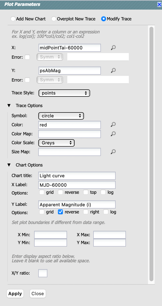
Plot parameters for the lightcurve.
3.3. View the i-band lightcurve for this SNIa.
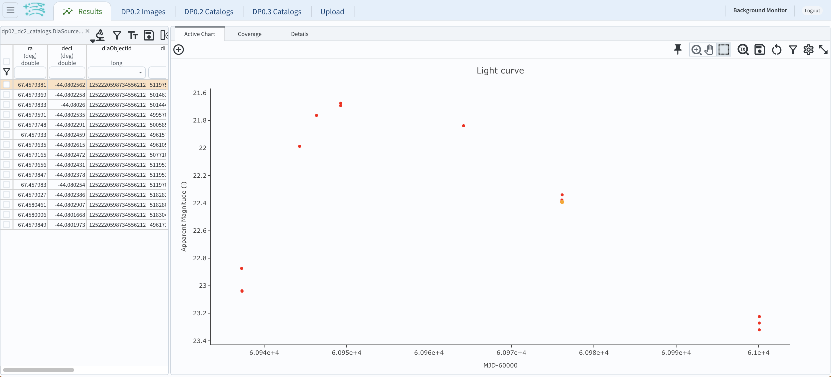
The i-band lightcurve for the SNIa of interest.
3.4. To add a plot of seeing versus time: click on the “+” sign on the upper-left corner of the active chart, and match the parameters shown below, then click “OK”.
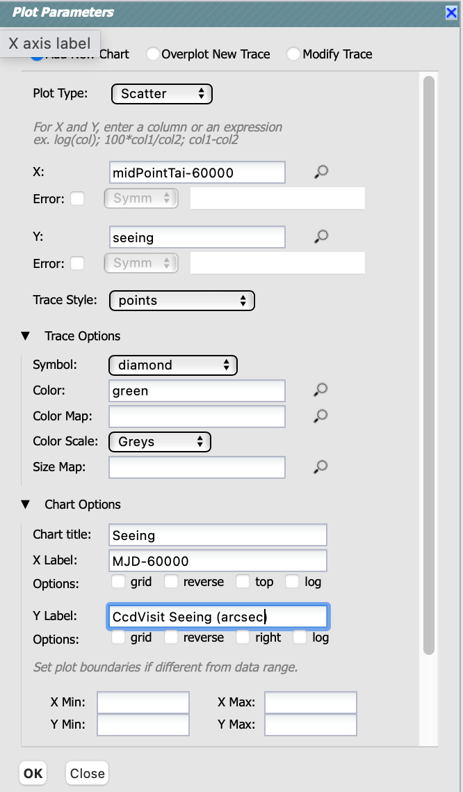
Plot parameters for the seeing versus time plot.
3.5. To add a plot to visualize the astrometric scatter: again, click on the “+” sign on the upper-left corner of the active chart, and match the parameters shown below, then click “OK”.
Note that in both the X and Y parameters, the difference between the DiaSource coordinate and the DiaObject coordinate are multiplied by 3600, so that the plot axes are in arcseconds: ((ra-67.4579634)*cos(decl*(pi()/180)))*3600 and (decl+44.080243)*3600.
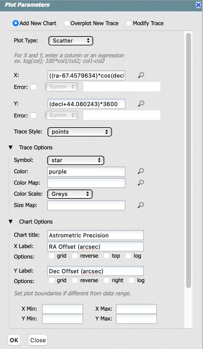
Plot parameters for the astrometric scatter plot.
3.6. View all three plots together. Plots might appear in a different order than as shown in the figure below. In the plot labeled “seeing”, click on the i-band epoch with the best seeing (0.75 arcsec). Notice how the point turns orange in all three plots, and that the corresponding table row will be highlighted.
In the lightcurve plot, notice that for this “best-seeing” epoch the SNIa had an apparent magnitude near its peak (around 22nd mag). That makes it a suitable choice for the scientific use-case outlined in the Introduction.
In the plot showing the astrometric scatter, notice that for this “bright / best-seeing” epoch the measured sky coordinates of the DiaSource are very close to those reported for the DiaObject. This does not necessarily mean that the coordinates for the “best-seeing” epoch are more accurate, because the coordinates of DiaObjects are derived from the individual DiaSources. The point of this plot is more that the overall scatter is less than 0.3 arcsec, and that selecting the “bright / best-seeing” epoch image for co-registration with images from other facilities is a wise choice.
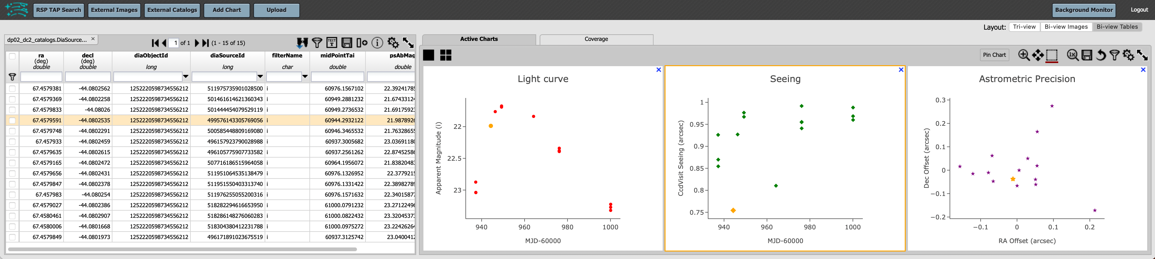
Identifying the best epoch for this scientific use-case.
4. Exercises for the learner
4.1. Obtain the visitId. At this point, the user is ready to obtain the “bright / best seeing” epoch’s images. The simplest way to do that is with the visitId, but the ADQL query did not request that from the CcdVisit table. Return to the ADQL query and add ccdvis.ccdVisitId and ccdvis.visitId to the query.
4.2. Add magnitude error bars.
To retrieve magnitude errors from the DiaSource catalog, return to step 2.2 and add to the ADQL statement:
scisql_nanojanskyToAbMagSigma(diasrc.psFlux, diasrc.psFluxErr) AS psAbMagErr.
When you get to step 3.1, for the Y error choose “Symm” from the drop-down menu, and then in the new box that appears to the right, enter “psAbMagErr”.
When you click “Apply” to create the plot, the points will have error bars.