01. Introduction to DP0.2 (beginner)
RSP Aspect: Notebook (terminal command-line)
Contact author: Gloria Fonseca Alvarez
Last verified to run: Sep 11 2023
LSST Science Pipelines version: Weekly 2023_35
Targeted learning level: Beginner
Container size: medium
Introduction: This tutorial is an introduction to the terminal and command line functionality within the Rubin Science Platform. It is parallel to the Jupyter Notebook tutorial “Introduction to DP02” and demonstrates how to use the TAP service to query and retrieve catalog data; matplotlib to plot catalog data; the LSST Butler package to query and retrieve image data; and the LSST afwDisplay image package.
This tutorial uses the Data Preview 0.2 (DP0.2) data set. This data set uses a subset of the DESC’s Data Challenge 2 (DC2) simulated images, which have been reprocessed by Rubin Observatory using Version 23 of the LSST Science Pipelines. More information about the simulated data can be found in the DESC’s DC2 paper and in the DP0.2 data release documentation.
Step 1. Access the terminal and setup
1.1. Log in to the Notebook Aspect. The terminal is a subcomponent of the Notebook Aspect.
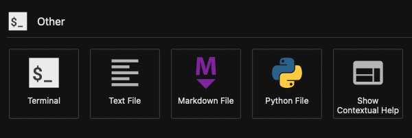
1.2. In the launcher window under “Other”, select the terminal.
1.3. Set up the Rubin Observatory environment.
setup lsst_distrib
1.4. Start an interactive Python session.
python
Step 2. Import packages
This tutorial makes use of several packages that will be commonly used when interacting with catalog and image data.
2.1. Import general python packages.
import numpy
import matplotlib
import matplotlib.pyplot as plt
2.2. Import packages needed to access the catalog data.
import pandas
pandas.set_option('display.max_rows', 1000)
from lsst.rsp import get_tap_service, retrieve_query
2.3. Import packages needed to access images.
import lsst.daf.butler as dafButler
import lsst.geom
import lsst.afw.display as afwDisplay
Step 3. Retrieve data using TAP for 10 objects
Table Access Procotol (TAP) provides standardized access to the catalog data for discovery, search, and retrieval. Full documentation for TAP is provided by the International Virtual Observatory Alliance (IVOA). The TAP service uses a query language similar to SQL (Structured Query Langage) called ADQL (Astronomical Data Query Language). The documentation for ADQL includes more information about syntax and keywords.
Notice: Not all ADQL functionality is supported by the RSP for Data Preview 0.
This example uses the DP0.2 Object catalog, which contains sources detected in the coadded images (also called stacked, combined, or deepCoadd images).
3.1. Start the TAP service .
service = get_tap_service("tap")
3.2. Define the coordinates for a cone search centered around the region covered by the DC2 simulation (RA,Dec = 62,-37).
use_center_coords = "62, -37"
3.3. Create a query named my_adql_query to retrieve the coordinates and g, r, i magnitudes for objects within 0.5 degrees of the center coordinates.
my_adql_query = "SELECT TOP 10 coord_ra, coord_dec, detect_isPrimary, " + \
             "r_calibFlux, r_cModelFlux, r_extendedness " + \
             "FROM dp02_dc2_catalogs.Object " + \
             "WHERE CONTAINS(POINT('ICRS', coord_ra, coord_dec), " + \
             "CIRCLE('ICRS', " + use_center_coords + ", 0.5)) = 1 "
3.4. Retrieve and display the results of the query for 10 objects.
results = service.search(my_adql_query)
results_table = results.to_table()
print(results_table)
3.5. Convert fluxes into magnitudes.
The object and source catalogs store only fluxes. There are hundreds of flux-related columns, and to store them also as magnitudes would be redundant, and a waste of space. All flux units are nanojanskys (nJy). To convert nJy to AB magnitudes use: mAB = -2.5log(fnJy) + 31.4.
Add columns of magnitudes after retrieving columns of flux.
results_table['r_calibMag'] = -2.50 * numpy.log10(results_table['r_calibFlux']) + 31.4
results_table['r_cModelMag'] = -2.50 * numpy.log10(results_table['r_cModelFlux']) + 31.4
Display the results table including the magnitudes.
print(results_table)
Step 4. Retrieve data using TAP for 10,000 objects
To retrieve columns of fluxes as magnitudes in an ADQL query, users can do this: scisql_nanojanskyToAbMag(g_calibFlux) as g_calibMag, and columns of magnitude errors can be retrieved with: scisql_nanojanskyToAbMagSigma(g_calibFlux, g_calibFluxErr) as g_calibMagErr.
4.1. Retrieve g-, r- and i-band magnitudes for 10000 point-like objects.
In addition to a cone search, impose query restrictions that detect_isPrimary is True (this will not return deblended “child” sources), that the calibrated flux is greater than 360 nJy (about 25th mag), and that the extendedness parameters are 0 (point-like sources).
results = service.search("SELECT TOP 10000 coord_ra, coord_dec, "
                        "scisql_nanojanskyToAbMag(g_calibFlux) as g_calibMag, "
                        "scisql_nanojanskyToAbMag(r_calibFlux) as r_calibMag, "
                        "scisql_nanojanskyToAbMag(i_calibFlux) as i_calibMag, "
                        "scisql_nanojanskyToAbMagSigma(g_calibFlux, g_calibFluxErr) as g_calibMagErr "
                        "FROM dp02_dc2_catalogs.Object "
                        "WHERE CONTAINS(POINT('ICRS', coord_ra, coord_dec), "
                        "CIRCLE('ICRS', "+use_center_coords+", 1.0)) = 1 "
                        "AND detect_isPrimary = 1 "
                        "AND g_calibFlux > 360 "
                        "AND r_calibFlux > 360 "
                        "AND i_calibFlux > 360 "
                        "AND g_extendedness = 0 "
                        "AND r_extendedness = 0 "
                        "AND i_extendedness = 0")
4.2. Store the data as a pandas dataframe.
results_table = results.to_table()
data = results_table.to_pandas()
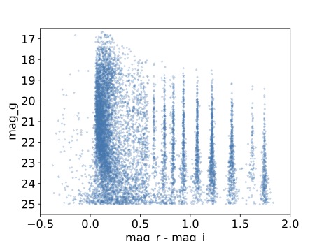
Step 5. Make a color-magnitude diagram
5.1. Plot the color (r-i magnitudes) vs g magnitude.
plt.plot(data['r_calibMag'].values - data['i_calibMag'].values,
     data['g_calibMag'].values, 'o', ms=2, alpha=0.2)
5.2. Define the axis labels and limits.
plt.xlabel('mag_r - mag_i', fontsize=16)
plt.ylabel('mag_g', fontsize=16)
plt.xticks(fontsize=16)
plt.yticks(fontsize=16)

plt.xlim([-0.5, 2.0])
plt.ylim([25.5, 16.5])
5.3. Save the plot as a pdf.
plt.savefig('color-magnitude.pdf')
Use the file navigator on the left-hand side of the Notebook Aspect to navigate to the file “color-magnitude.pdf”. Double click on the filename to open and view the plot.
Step 6. Retrieve image data using the butler
The two most common types of images that DP0 users will interact with are calexps and deepCoadds.
calexp: A single image in a single filter.
deepCoadd: A combination of single images into a deep stack or Coadd.
The LSST Science Pipelines processes and stores images in tracts and patches. To retrieve and display an image at a desired coordinate, users have to specify their image type, tract, and patch.
tract: A portion of sky within the LSST all-sky tessellation (sky map); divided into patches.
patch: A quadrilateral sub-region of a tract, of a size that fits easily into memory on desktop computers.
The butler (butler documentation) is an LSST Science Pipelines software package to fetch LSST data without having to know its location or format. The butler can also be used to explore and discover what data exists. Other tutorials demonstrate the full butler functionality.
6.1. Define a butler configuration and collection.
butler = dafButler.Butler('dp02', collections='2.2i/runs/DP0.2')
6.2. Define the coordinates of a known galaxy cluster in the DC2.
my_ra_deg = 55.745834
my_dec_deg = -32.269167
6.3. Use lsst.geom to define a SpherePoint for the cluster’s coordinates (lsst.geom documentation).
my_spherePoint = lsst.geom.SpherePoint(my_ra_deg*lsst.geom.degrees, my_dec_deg*lsst.geom.degrees)
print(my_spherePoint)
6.3. Retrieve the DC2 skymap (skymap documentation) and identify the tract and patch.
skymap = butler.get('skyMap')
tract = skymap.findTract(my_spherePoint)
patch = tract.findPatch(my_spherePoint)

my_tract = tract.tract_id
my_patch = patch.getSequentialIndex()

print('my_tract: ', my_tract)
print('my_patch: ', my_patch)
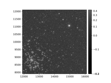
6.4. Retrieve the deep i-band Coadd.
dataId = {'band': 'i', 'tract': my_tract, 'patch': my_patch}
my_deepCoadd = butler.get('deepCoadd', dataId=dataId)
Step 7. Display the image
Image data retrieved with the butler can be displayed several different ways.
7.1. Display the image using afwDisplay (afwDisplay documentation).
afwDisplay.setDefaultBackend('matplotlib')
fig = plt.figure(figsize=(10, 8))
afw_display = afwDisplay.Display(1)
afw_display.scale('asinh', 'zscale')
afw_display.mtv(my_deepCoadd.image)
plt.gca().axis('on')
plt.savefig('my_deepCoadd.pdf')
Use the file navigator on the left-hand side of the Notebook Aspect to navigate to the file “my_deepCoadd.pdf”. Double click on the filename to open and view the image.
7.2. Display the image using Firefly (Firefly documentation).
afwDisplay.setDefaultBackend('firefly')
afw_display = afwDisplay.Display(frame=1)
afw_display.mtv(my_deepCoadd)
Optional: For a demonstration of the Firefly interactive interface, work through “03b Image Display with Firefly” of the Notebook tutorials.
7.3. When you’re done, exit python to return to the regular command line.
exit()